Definite Integrals for Area Between Curves and for Average Value of a Function

Section 4.2 Definite Integrals for Area Between Curves and for Average Value of a Function

In this section, we briefly review (from the first calculus course) the main idea behind setting up a definite integral that represents the area of a region between two curves. We will re-use this main idea several times during this course, for different settings and different interpretations of the definite integral. We also review setting up the definite integral to compute the average value of a function on an interval.

🔗

Subsection 4.2.1 Review of Area Between Curves

🔗

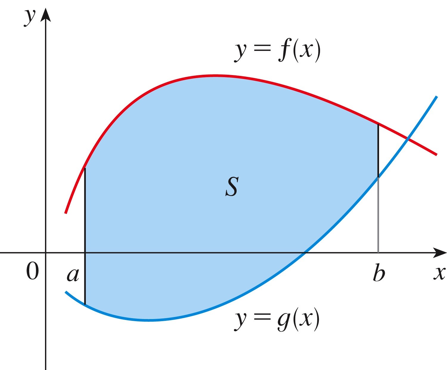
Consider the region

S

$S$ shown in the figure below. The region is bounded above by the graph of

y = f (x),

$y=f(x)\text{,}$ below by the graph of

y = g (x),

$y = g(x)\text{,}$ to the left by the vertical line

x = a,

$x=a\text{,}$ and to the right by the vertical line

x = b .

$x=b\text{.}$

🔗

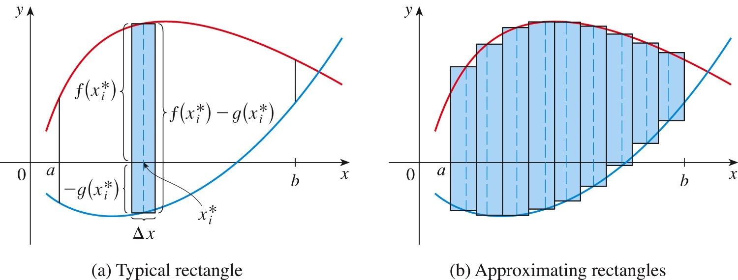
Calculating

A,

$A\text{,}$ the area of region

S,

$S\text{,}$ is very similar to calculating the area under a curve, as shown in the figure below:

We divide the interval $[a,b]$ into $n$ subintervals of equal width $\displaystyle \Delta x = \frac{b-a}{n}\text{.}$
On each subinterval, we build an approximating rectangle with base $\Delta x\text{.}$
The height of the $i$ th approximating rectangle is $f(x_i^*) - g(x_i^*)\text{.}$
The area of the $i$ th approximating rectangle is height times width, that is, $\left[ f(x_i^*) - g(x_i^*) \right] \Delta x\text{.}$
The total area of all $n$ approximating rectangles is $\displaystyle \sum_{i=1}^n \left[ f(x_i^*) - g(x_i^*) \right] \Delta x\text{.}$
The total area $A$ then is the limiting value of the latter, namely $A = \lim_{n \to \infty} \sum_{i=1}^n \left[ f(x_i^*) - g(x_i^*) \right] \Delta x = \int_a^b \left[ f(x) - g(x) \right] \ dx.$

🔗
Figure The approximate area of region $S$ is the sum of the areas of all approximating rectangles. Source: Biocalculus: Calculus for the Life Sciences, James Stewart and Troy Day, Cengage Learning, 2015.

🔗

Subsection 4.2.2 Shortcut for Setting up a Definite Integral for Area Between Curves: Focus on a Typical Slice

🔗

The notation used above, with superscripts

$*\text{,}$ subscripts

$i\text{,}$

$\displaystyle \sum_{i=1}^n\text{,}$ and

$\displaystyle \lim_{n \to \infty}$ is rather cumbersome, especially knowing that it all goes away in the last step when writing the definite integral. Ideally, we find a way to construct the definite integral without all that cumbersome notation!

🔗

In the simplified construction process, we focus on a typical slice of width

$dx$ (similar to focussing on the

$i$ th approximating rectangle with width

$\Delta x$ as we did above).

🔗

In the following video, we show how to construct the definite integral for the area between two curves by focussing on a typical slice.

🔗

Figure 4.2.3. Video demonstrating the construction of a definite integral to represent the area between two curves by focussing on a typical slice of width

$dx\text{.}$

🔗

While it may be tempting to "memorize" the form of the definite integral for the area between two curves, it is helpful to use the simplified construction process with a typical slice.

🔗

This simplified construction process generalizes nicely to other applications of the definite integral (we will encounter these shortly), such as calculating the mass of an object with varying density or calculating the volume of a three-dimensional object.

🔗

In all cases, the underlying idea is the same: we chop or make slices and add things up (whether we add the areas or masses or volumes of the slices).

🔗

Subsection 4.2.3 Definite Integral for the Average Value of a Function

🔗

Many quantities are continuous. Examples include temperature at the Edmonton International Airport (as a function of time) and blood glucose concentration in a diabetic patient (as a function of time). How would we calculate their average values over a period of time?

🔗

We know how to calculate the average of

$n$ numbers,

$y_1\text{,}$

$y_2\text{,}$

$\ldots\text{,}$

$y_n\text{.}$ We add them up, and divide by

$n\text{:}$

$y_{ave} = \frac{ y_1 + y_2 + \ldots + y_n }{ n }.$ To generalize this to the concept of an average value of a function, slicing (or chopping) again is going to be the key.

🔗

In the following video, we show how the average value of a function is defined in terms of a definite integral, and work through a biological application.

🔗

Figure 4.2.4. Video developing the definite integral representing the average value of a function.

🔗

Subsection 4.2.4 The Mean Value Theorem for Integrals

🔗

It seems reasonable to think that there is a function value in the interval

$[a,b]$ that is exactly equal to the average value of the function over the interval

$[a,b]\text{.}$ The Mean Value Theorem for Integrals guarantees that this is indeed the case (under the usual condition that the function is continuous).

🔗

In the following video, we introduce the Mean Value Theorem for Integrals, and give a geometric interpretation.

🔗

Figure 4.2.5. Video on the Mean Value Theorem for Integrals.

🔗

Subsection 4.2.5 Summary

🔗

Area Between Curves.

The area $A$ of the region bounded by the curves of continuous functions $y = f(x)$ and $y = g(x)\text{,}$ and the vertical lines $x=a$ and $x=b\text{,}$ where $f(x) \ge g(x)$ for all $x$ in $[a,b]\text{,}$ is $A = \int_a^b \left[ f(x) - g(x) \right] \ dx.$

🔗

Average Value of a Function.

The average value of a function $y=f(x)$ on the interval $[a,b]$ is $f_{ave} = \frac{1}{b-a} \int_a^b f(x) \ dx.$

🔗

The Mean Value Theorem for Integrals.

If $f$ is continuous on the interval $[a,b]\text{,}$ then there exists a number $c$ such that $f(c) = f_{ave} = \frac{1}{b-a} \int_a^b f(x) \ dx,$ that is, $\int_a^b f(x) \ dx = f(c) \dot (b-a).$

🔗

Subsection 4.2.6 Don't Forget

🔗

Don't forget to return to eClass to complete the pre-class quiz.

🔗

Subsection 4.2.7 Further Study

🔗

Remember that the notes presented above only serve as an introduction to the topic. Further study of the topic will be required. This includes working through the pre-class quizzes, reviewing the lecture notes, and diligently working through the homework problems.

🔗

As you study, you should reflect on the following learning outcomes, and critically assess where you are on the path to achieving these learning outcomes:

🔗

Learning Outcomes

Set up the definite integral that represents the area of a given planar region.
Set up and evaluate the definite integral that represents the average value of a given function over a given integral.
Recall the statement of the Mean Value Theorem for Integrals and interpret its meaning geometrically.

🔗

The following references provide a good start for review and further study:

Learning Outcome	Video	Textbook Section
1	4.E4	6.1
2	4.E5	6.2
3	4.E6	6.2