Section 9.1 Systems of Differential Equations
In this notebook, we introduce the concept of a system of coupled differential equations. Almost any phenomenon observed in the real world results from the interactions of multiple factors. For example, in a predator-prey system (wolves and rabbits, ladybugs and aphids, etc), two species interact. A decline in the prey population affects the predator population and vice versa.
We limit our attention to systems of two autonomous differential equations and the visualization of the solutions in the phase plane.
Subsection 9.1.1 Parametric Curves
We make a brief detour to introduce the concept of a parametric curve. We will see later that solutions of systems of autonomous differential equations can be represented as parametric curves.
Suppose that \(x\) and \(y\) are both functions of time \(t\text{,}\) that is, they are defined by the equations $$x = f(t) \ \ \text{and} \ \ y = g(t).$$
Each value of \(t\) determines a point \((x,y)\) that we can plot in the coordinate plane. As \(t\) varies, the point \((x,y) = (f(t), g(t))\) also varies and traces a curve in the coordinate plane. Such curve is called a parametric curve. The equations \(x = f(t)\) and \(y = g(t)\) are called parametric equations.
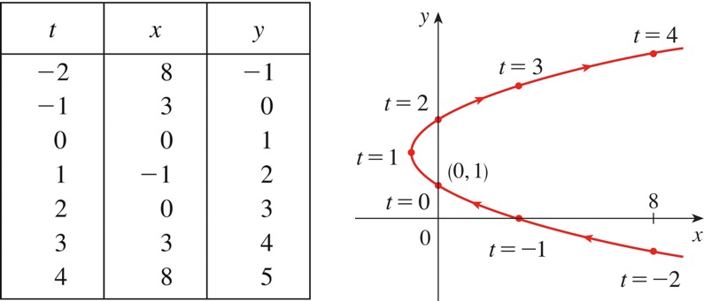
For example, suppose we have parametric equations \(x = t^2 - 2t\) and \(y = t+1\text{.}\) The table shown below shows the values of \(x\) and \(y\) for various values of \(t\text{,}\) and the figure shown below shows the resulting parametric curve in the coordinate plane. Note that the direction of the movement as \(t\) increases is indicated with arrows.
Subsection 9.1.2 A System of Two Differential Equations
Consider a system of two autonomous differential equations
A solution of this system of differential equations is a pair of functions \(x(t)\) and \(y(t)\) that simultaneously satisfy the two differential equations.
To visualize the solution, it is helpful to show both of the following:
- The graph of \(x(t)\) versus \(t\) and the graph of \(y(t)\) versus \(t\text{.}\)
- The graph of \(y(t)\) vs \(x(t)\text{,}\) that is, the parametric curve in the \((x,y)\) plane. In the context of a system of differential equations, the \((x,y)\) plane is also known as the phase plane.
Subsection 9.1.3 The Love Affair of Romeo and Juliet
By way of example, consider the relationship between two lovers, Romeo and Juliet. It is reasonable to expect that their relationship will be dynamic. That is, we expect Romeo and Juliet's feelings for each other to change over time. Moreover, Romeo and Juliet influence each other's feelings.
We seek a mathematical model that describes Romeo and Juliet's feelings over time. First, consider Romeo's feelings towards Juliet. Because we are interested in Romeo's feelings over time, let us denote Romeo's feelings towards Juliet at time \(t\) by \(R(t)\text{.}\)
- When \(R(t) \gt 0\text{,}\) Romeo loves Juliet.
- When \(R(t) = 0\text{,}\) Romeo is neutral towards Juliet.
- When \(R(t) \lt 0\text{,}\) Romeo hates Juliet (more nicely put, he does not like her, or has negative feelings towards her).
- The larger the value of \(|R|\text{,}\) the more intense the feeling of love or hate.
Similarly, we denote Juliet's feelings towards Romeo at time \(t\) by \(J(t)\text{.}\)
Our model will consist of differential equations for \(R(t)\) and \(J(t)\text{.}\) Let's start by writing a simple differential equation for \(R(t)\text{.}\) For now, assume that Romeo responds to his own feelings according to $$ \frac{dR}{dt} = a_R R, $$ where \(a_R\) is a parameter.
We recognize this differential equation as the World's Most Important Differential Equation. Its solution is $$ R(t) = R_0 e^{a_R t}, $$ where \(R_0\) is Romeo's initial feelings.
- If \(a_R \gt 0\text{,}\) then Romeo's initial feelings for Juliet intensify (exponential growth to positive or negative infinity, depending on the sign of \(R_0\text{;}\) if Romeo loves Juliet initially, he will love her more and more over time; if he hates her initially, he will hate her more and more over time). This case can be interpreted as representing the saying absence makes the heart grow fonder.
- If \(a_R \lt 0\text{,}\) Romeo's initial feelings for Juliet fizzle (exponential decay to zero; Romeo becomes neutral towards Juliet over time). This case can be interpreted as representing the saying out of sight, out of mind.
Similarly, we can assume that Juliet responds to her own feelings according to $$ \frac{dJ}{dt} = a_J J, $$ where \(a_J\) is a parameter. This means that Juliet's feelings also either intensify (if \(a_J \gt 0\)) or fizzle (if \(a_J \lt 0\)).
So far, we do not have a system of differential equations yet, but two independent differential equations. How Romeo's feelings develop depends only on his own feelings, and is independent of Juliet's feelings for him. To reflect how Romeo responds to Juliet's feelings for him, the equation for \(R\) must depend on \(J\text{;}\) similarly, to reflect how Juliet responds to Romeo's feeling for her, the equation for \(J\) must depend on \(R\text{.}\) We modify the original two differential equations as follows:
where \(p_R\) and \(p_J\) are parameters that describe how Romeo responds to Juliet's feelings for him and how Juliet responds to Romeo's feelings for him, respectively. The parameters \(a_R\) and \(a_J\) have the same meaning as before.
Remark 9.1.2.
Note that Romeo's parameters have the subscript \(R\text{,}\) and Juliet's parameters have the subscript \(J\text{.}\) The parameters \(a_R\) and \(a_J\) represent Romeo's and Juliet's response to their own feelings for the other (in the absence of the other), respectively, while the parameters \(p_R\) and \(p_J\) represent Romeo's and Juliet's response to the other's feelings for them (in the presence of the other), respectively.The outcome of Romeo and Juliet's relationship depends on their romantic styles, encoded in the value of the parameters \(a_R\text{,}\) \(a_J\text{,}\) \(p_R\text{,}\) and \(p_J\text{,}\) and their initial feelings for each other, encoded in the initial conditions \(R(0)\) and \(J(0)\text{.}\)
In the following examples, we examine the outcome of the relationship for six sets of parameters. For each case, the initial conditions were set to \(R(0)=1\) and \(J(0)=1\text{.}\)
In the following examples, the upper graph is a plot of the solution, \(R(t)\) and \(J(t)\text{,}\) in blue and pink, respectively. The lower graph is a plot of the solution in the \((R,J)\) phase plane. For each case, examine the relationship between the solution in the upper and lower graphs. Note that the solutions in the lower graphs are missing the arrows indicating the direction of increasing \(t\text{.}\) Can you determine the direction of the arrows?
Remark 9.1.3.
Readers who are savvy on the computer and have some extra time on their hands may wish to experiment with this Romeo and Juliet simulation tool. It is a Flash applet, which is outdated technology (most browsers have stopped supporting Flash). However, there are some apps available that can run Flash applets. For example, a good app for the Mac that can handle Flash applets is the free Elmedia Video Player.
Example 9.1.4. Case Study 1.
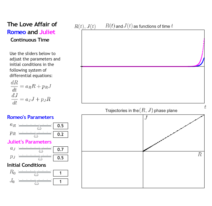
As \(t \to \infty\text{,}\) both \(R(t)\) and \(J(t) \to \infty\text{.}\)
For this case, Romeo and Juliet's relationship lasts forever, in a positive sense: Romeo's love for Juliet and Juliet's love for Romeo become stronger over time.
The arrows point towards the upper right corner of the phase plane.
Example 9.1.6. Case Study 2.
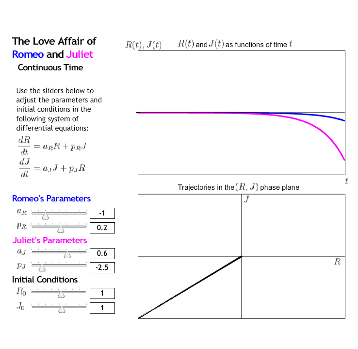
As \(t \to \infty\text{,}\) both \(R(t)\) and \(J(t) \to -\infty\text{.}\)
For this case, Romeo and Juliet's relationship lasts forever, but in a very negative sense: Romeo's initial love for Juliet and Juliet's initial love for Romeo quickly become feelings of hate, which become stronger over time.
The arrows point towards the lower left corner of the phase plane.
Example 9.1.8. Case Study 3.
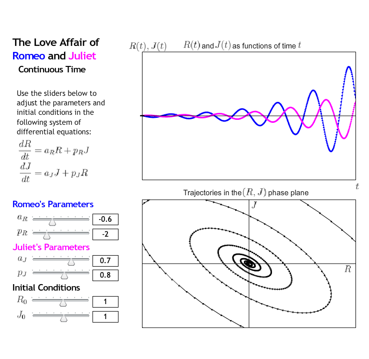
As \(t \to \infty\text{,}\) Romeo and Juliet's relationship becomes increasingly tumultuous. This is apparent by the growing oscillation.
For this case, Romeo and Juliet's relationship lasts forever in the sense that they do not eventually feel neutral towards each other. However, since both \(R(t)\) and \(J(t)\) oscillate, we see that Romeo and Juliet express both love and hate for each other. Their feelings are mutually loving approximately one quarter of the time.
The arrows point in the counterclockwise direction.
Example 9.1.10. Case Study 4.
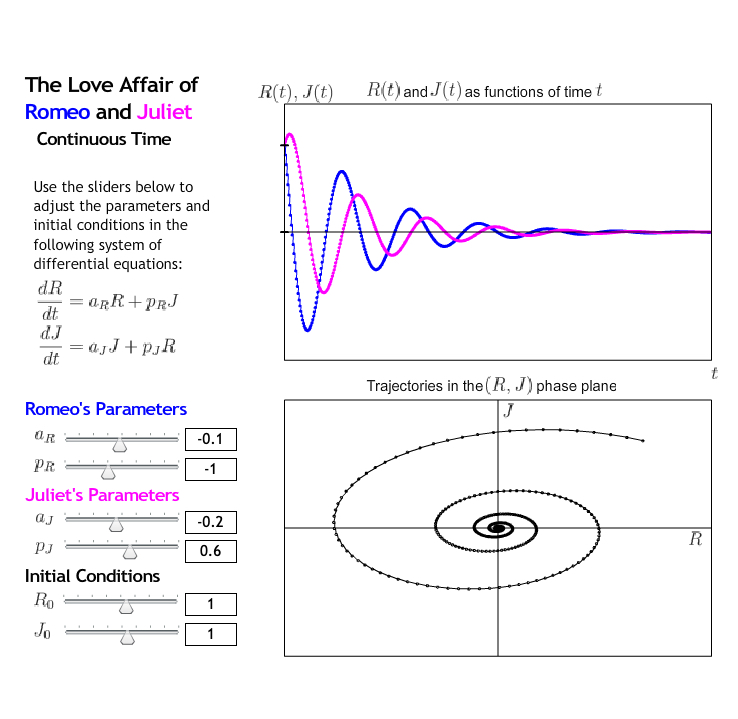
As \(t \to \infty\text{,}\) both \(R(t)\) and \(J(t) \to 0\text{.}\)
For this case, Romeo and Juliet's relationship does not last; they eventually feel neutral towards each other. They both start out in love, but quickly begin to hate each other. Shortly after, they fall back in love, but less intensely. This cycle continues, with their feelings towards each other becoming less intense as time goes on.
The arrows point in the counterclockwise direction.
Example 9.1.12. Case Study 5.
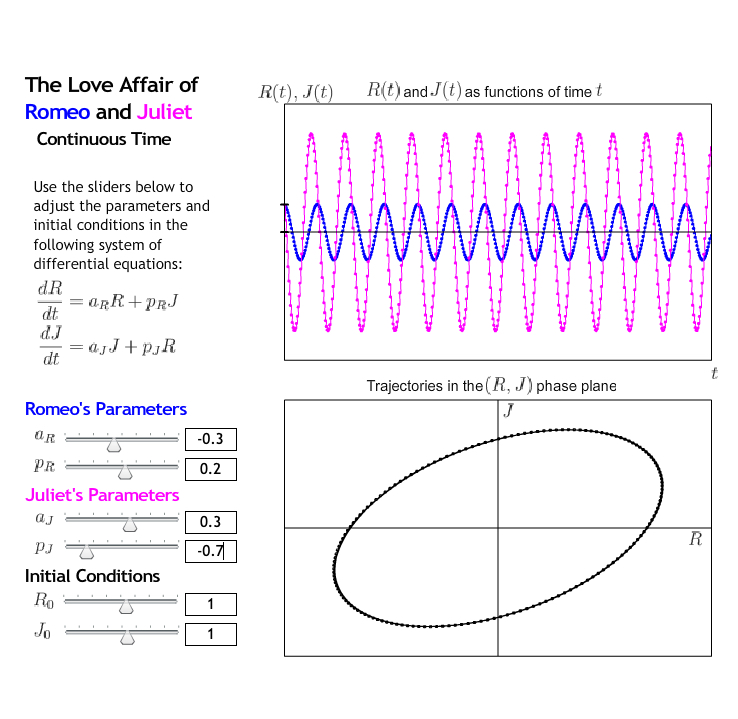
For this case, Romeo and Juliet have a tumultuous relationship. Their feelings consistently oscillate between love and hate. It is important to note that the intensity of their mood swings does not change. In other words, their relationship is periodic. This can be seen by looking at the solution in the phase plane and observing the elliptical solution. As opposed to the spiral solutions from Case Studies 3 and 4, we observe a solution that forms a closed loop.
This relationship lasts. In fact, Romeo and Juliet have very predictable feelings. Both \(R(t)\) and \(J(t)\) continue to oscillate forever, much like the sine and cosine functions.
The arrows point in the clockwise direction. It is a little trickier to see this here than for Case Studies 3 and 4. To see it, focus on the first local minimum of the pink curve in the upper graph. This point corresponds to the bottom-most point on the ellipse in the lower graph (where \(J(t)\) is at its most negative). As time increases, the pink curve or \(J(t)\) increases in the upper graph. In the lower graph, this corresponds to moving up from the bottom-most point on the ellipse. To determine whether the solution moves clockwise or counterclockwise, we need to take a look at what the blue curve or \(R(t)\) is doing in the upper graph. If you look closely, you should see that \(R(t)\) continues to decrease before it reaches its minimum. On the lower graph then, decreasing \(R(t)\) corresponds to moving to the left along the ellipse. That is, the solution is going clockwise, and the arrows point in the clockwise direction.
Subsection 9.1.4 Summary
Parametric Equations and Parametric Curves.
- Parametric equations represent variables that depend on a parameter (or multiple parameters). In the context of differential equations in MATH 136, parametric equations depend on only one parameter, and the parameter most often is time \(t\text{.}\)
- A parametric curve is a curve that is defined parametrically; it is the curve traced out in variable space as the parameter is varied.
Systems of (Autonomous) Differential Equations.
-
For the following system of two autonomous differential equations:
\begin{alignat*}{1} \frac{dx}{dt} &= f(x,y) \\ \frac{dy}{dt} &= g(x,y) \end{alignat*}- A solution is the pair of functions \(x(t)\) and \(y(t)\) that simultaneously satisfy the differential equations.
- The phase plane is the \((x,y)\) plane; the phase plane is used to represent solutions of the system of differential equations as parametric curves.
Subsection 9.1.5 Don't Forget
Don't forget to return to eClass to complete the pre-class quiz.
Subsection 9.1.6 Further Study
Remember that the notes presented above only serve as an introduction to the topic. Further study of the topic will be required. This includes working through the pre-class quizzes, reviewing the lecture notes, and diligently working through the homework problems.
As you study, you should reflect on the following learning outcomes, and critically assess where you are on the path to achieving these learning outcomes:
Learning Outcomes
- Recognize the solution of a system of two autonomous differential equations as parametric equations.
- Represent the solution of a system of two autonomous differential equations as a parametric curve in the phase plane.
The following references provide a good start for review and further study:
| Learning Outcome | Video | Textbook Section |
|---|---|---|
| 1 | N/A | 7.5 |
| 2 | N/A | 7.5 |