Section 11.1 Exponential and Normal Random Variables
Subsection 11.1.1 Exponential Random Variables
Exponential random variables are used in situations involving a waiting time. Examples include waiting for a service representative to answer our phone call, or waiting for the LRT to arrive at University Station. Biological examples include a predator waiting for a prey to arrive, or waiting for a new drug therapy to be developed.
In general, an exponential random variable \(T\) with positive parameter \(c\) takes on values from the set \([0, \infty)\) and has probability density function
It is a straightforward exercise (using integration by parts; left to the reader) to show that the expected value or mean of \(T\) is $$ E[T] = \mu = \int_{-\infty}^{\infty} t f(t) \ dt = c \int_0^{\infty} t e^{-ct} \ dt = \frac{1}{c}. $$
We therefore can rewrite the probability density function in terms of the mean \(\mu\text{,}\) as follows:
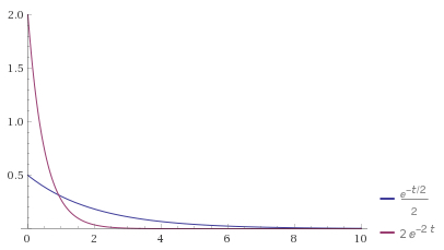
The graphs of the probability density functions for two exponential random variables are shown below, for \(\mu = 2\) and \(\mu = 1/2\text{.}\) Note that the larger the value of \(\mu\text{,}\) the slower the exponential decay to zero.

plot 1/2 e^(-1/2 t) and 2 e^(-2t), t=0..10, y=0..2.In the following video, we work through an example using the exponential random variable.
Subsection 11.1.2 Normal Random Variables
Normal random variables are used in situations where many independent factors influence an outcome. Typical applications are to describe the characteristics of an individual or organism (such as the height of a MATH 136 student, determined by a combination of genetic, developmental, and environmental factors), tests results (such as MCAT scores), or measurement errors.
A normal random variable \(X\) with mean \(\mu\) and standard deviation \(\sigma\) has probability density function $$ f(x) = \frac{1}{\sigma \sqrt{2 \pi}} e^{ -\frac{1}{2} \left( \frac{x-\mu}{\sigma} \right)^2}. $$
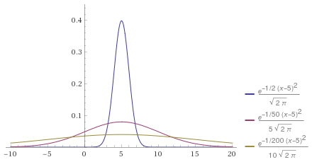
The graphs of the probability density function for three normal random variables with the same mean \(\mu = 5\) but different standard deviations \(\sigma\) (\(\sigma =\) 1, 5, and 10) are shown below. Note that the probability density functions are symmetric about the mean \(\mu\text{.}\) Further, the smaller the value of the standard deviation \(\sigma\text{,}\) the more tightly clustered the values of \(X\) are about the mean (the larger the value of the standard deviation \(\sigma\text{,}\) the larger the spread of the values of \(X\)).

plot { 1\(1 sqrt(2 pi)) e^( -1/2 ((x-5)/1)^2 ), 1\(5 sqrt(2 pi)) e^( -1/2 ((x-5)/5)^2 ), 1\(10 sqrt(2 pi)) e^( -1/2 ((x-5)/10)^2 ) }, x=-10..20, y=0..0.45.In the following video, we work through an example using the normal random variable.
Subsection 11.1.3 Summary
Exponential Random Variables.
- An exponential random variable \(T\) with mean \(\mu\) has probability density function\begin{equation*} f(t) = \begin{cases} \frac{1}{\mu} e^{-\frac{1}{\mu} t} \amp \text{for } t \ge 0 \\ 0 \amp \text{for } t \lt 0. \end{cases} \end{equation*}
Normal Random Variables.
- A normal random variable \(X\) with mean \(\mu\) and standard deviation \(\sigma\) has probability density function $$ f(x) = \frac{1}{\sigma \sqrt{2 \pi}} e^{ -\frac{1}{2} \left( \frac{x-\mu}{\sigma} \right)^2}. $$
Subsection 11.1.4 Don't Forget
Don't forget to return to eClass to complete the pre-class quiz.
Subsection 11.1.5 Further Study
Remember that the notes presented above only serve as an introduction to the topic. Further study of the topic will be required. This includes working through the pre-class quizzes, reviewing the lecture notes, and diligently working through the homework problems.
As you study, you should reflect on the following learning outcomes, and critically assess where you are on the path to achieving these learning outcomes:
Learning Outcomes
- Construct the probability density function of an exponential random variable with given mean, and apply it to determine the probability of a given event by evaluating an appropriate definite or improper integral.
- Construct the probability density function of a normal random variable with given mean and standard deviation, and use technology to determine the probability of a given event.
- Sketch graphs of the probability density function of the normal distribution for different means and standard deviations.
- Rewrite probability events involving a normal distribution in terms of the standard normal distribution, and use the \(z\)-score table to determine the probability of the event.
The following references provide a good start for review and further study:
| Learning Outcome | Video | Textbook Section |
|---|---|---|
| 1 | 11.E1 | 12.5 |
| 2 | 11.E2 | 12.5 |
| 3 | N/A | 12.5 |
| 4 | N/A | 12.5 |