Section 7.2 Qualitative Analysis of Differential Equations
It is not always possible or necessary to determine the solution of the differential equation explicitly (in closed form, or in terms of elementary functions). However, it often suffices to determine the qualitative nature of the solutions.
In this section, we will learn techniques to carry out a qualitative analysis of autonomous differential equations and their solutions. This analysis is referred to as phase plot analysis.
Remark 7.2.1.
Students who have taken MATH 134 already will be familiar with phase plot analysis, but may benefit from a review of this topic.Subsection 7.2.1 Autonomous Differential Equations
An autonomous differential equation is a differential equation that relates an unknown function and its derivatives, but without an explicit dependence on the independent variable (such as time). Autonomous differential equations have the form $$\frac{dy}{dt} = f(y),$$ where \(f(y)\) is given, \(y\) is the unknown function or dependent variable, and \(t\) is the independent variable. Note that \(f(y)\) often also involves on one or more parameters.
Checkpoint 7.2.2.
Checkpoint 7.2.3.
Subsection 7.2.2 Phase Plot Analysis
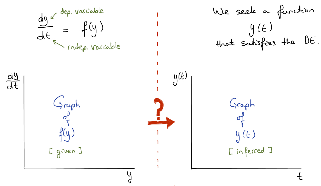
Phase plot analysis is a graphical analysis of an autonomous differential equation in the form $$\frac{dy}{dt} = f(y).$$ Recall that we seek functions \(y(t)\) that satisfy the differential equation. Phase plot analysis facilitates the visualization of the qualitative nature of the family of solutions, \(y(t)\text{.}\) It starts with the graph of \(f(y)\text{,}\) and ends with qualitative graphs of \(y(t)\text{,}\) as summarized in the following figure:

Given the graph of \(\displaystyle \frac{dy}{dt} = f(y)\) versus \(y\) on the left, we aim to infer qualitative sketches of the family of solutions, that is, we aim to infer the graph of \(y(t)\) versus \(t\) on the right.
Remark 7.2.5.
This is a challenging concept. Do take a moment to understand the difference between the two graphs, taking particular notice of the labels on the horizontal and vertical axes.Phase plot analysis brings together the following statements to infer the graph of \(y(t)\) versus \(t\text{:}\)
- Whenever \(f(y) \gt 0\text{,}\) \(\displaystyle \frac{dy}{dt} \gt 0\text{,}\) and so \(y(t)\) increases.
- Whenever \(f(y) \lt 0\text{,}\) \(\displaystyle \frac{dy}{dt} \lt 0\text{,}\) and so \(y(t)\) decreases.
- Whenever \(f(y) = 0\text{,}\) \(\displaystyle \frac{dy}{dt} = 0\text{,}\) and so \(y(t)\) does not change.
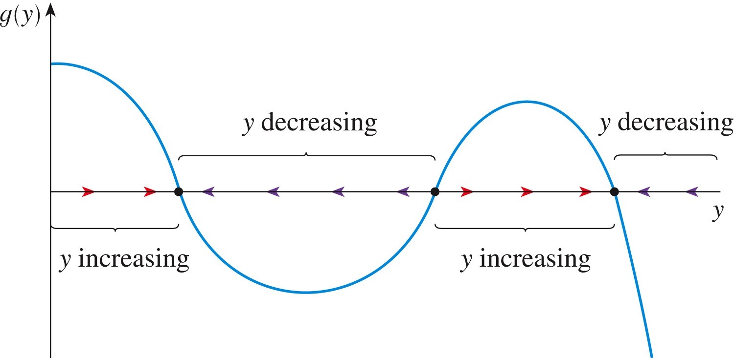
The following figure summarizes the above statements graphically, with arrows on the horizontal axis indicating whether \(y\) increases (by arrows pointing to the right) or decreases (by arrows pointing to the left), and with bullet points indicating where \(y\) does not change. Note that the figure refers to \(g(y)\) instead of \(f(y)\text{.}\)

Remark 7.2.7.
The last figure completes the first half of phase plot analysis. It provides the basis for completing the second half of phase plot analysis, which is to infer the qualitative nature of the graph of \(y(t)\text{.}\)In the following video (from MATH 134), we take you through phase plot analysis for a couple of examples.
Subsection 7.2.3 Phase Plot Analysis of the Logistic Equation
The Logistic Equation perhaps is the second-most important differential equation (after the World's Most Important Differential Equation, which represents exponential growth and decay), at least in the context of modelling in the life sciences.
While exponential growth (or decay) is a reasonable model for some situations, such as the initial growth of a population, or the initial growth of the number of infected individuals in a population in the context of an infectious disease spreading through the population, eventually the exponential model no longer applies. For example, at a certain size, a growing population will reach a limit where the habitat will not support any more individuals. The Logistic Equation models this situation, namely limited growth.
Suppose that the per-capita growth rate of a population of size \(N\) declines linearly from a value of \(r\) when \(N=0\) to a value of 0 when \(N=K\text{,}\) where \(K\) is the carrying capacity of the environment, then $$\frac{dN/dt}{N} = r \left( 1 - \frac{N}{K} \right),$$ where \(N(t)\) is the size of the population at time \(t\text{.}\) The left-hand side of the equation expresses the per-capita growth rate (growth rate \(dN/dt\) divided by the number of individuals in the population), and the right-hand side of the equation expresses the linear decrease in the per-capital growth rate as a function of \(N\text{.}\) When \(N=0\text{,}\) the per-capita growth rate is \(r\text{;}\) when \(N=K\text{,}\) the per-capita growth rate is \(K\text{.}\)
Rewriting the equation, we obtain the Logistic Equation, namely $$\frac{dN}{dt} = r N \left( 1 - \frac{N}{K} \right)$$ or $$\frac{dN}{dt} = \frac{r}{K} N \left( K - N \right).$$ We recognize the Logistic Equation as a differential equation, where \(t\) is the independent variable, \(N\) is the dependent variable, and \(r\) and \(K\)are parameters (that may vary from one population or environment to another).
Remark 7.2.9.
Visit the Wikipedia page on the Logistic Equation to learn more about the applicability of the Logistic Equation in a wide variety of scientific and social disciplines.The Logistic Equation is an autonomous differential equation, so it is amenable to phase plot analysis. In the following video, we will carry out the phase plot analysis for the case \(\displaystyle r = \frac{3}{2}\) and \(K = 4000\text{,}\) that is, for the differential equation $$\frac{dN}{dt} = \frac{3}{2} N \left( 1 - \frac{N}{4000} \right).$$
Subsection 7.2.4 Equilibria, Stability, and the Local Stability Criterion
We will cover this material in class.
Subsection 7.2.5 Summary
Autonomous Differential Equations.
- Autonomous differential equations are those that involve the derivative of an unknown function (the dependent variable) and the function itself, but not the independent variable.
- An autonomous differential equation has the form $$\frac{dy}{dt} = f(y).$$
Phase Plot Analysis.
- Phase plot analysis facilitates the visualization of the qualitative nature of solutions to autonomous differential equations, as well as the determination of equilibria and their stability.
-
A phase plot shows the graph of \(\displaystyle \frac{dy}{dt} = f(y)\) versus \(y\text{.}\)
- Whenever \(f(y) \gt 0\text{,}\) \(\displaystyle \frac{dy}{dt} \gt 0\text{,}\) and so \(y(t)\) increases.
- Whenever \(f(y) \lt 0\text{,}\) \(\displaystyle \frac{dy}{dt} \lt 0\text{,}\) and so \(y(t)\) decreases.
- Whenever \(f(y) = 0\text{,}\) \(\displaystyle \frac{dy}{dt} = 0\text{,}\) and so \(y(t)\) does not change.
The Logistic Equation.
- The Logistic Equation is $$\frac{dN}{dt} = r N \left( 1 - \frac{N}{K} \right),$$ where \(r\) is a per-capita growth rate, and \(K\) is the carrying capacity.
- The Logistic Equation is an autonomous differential equation that is amenable to phase plot analysis.
- The Logistic Equation is a separable differential equation that can be solved explicitly for \(N(t)\) using the method of partial fractions.
Equilibria and Stability.
- An equilibrium of the autonomous differential equation $$\frac{dy}{dt} = f(y)$$ is a constant value of \(y\) (denoted \(\hat{y}\)) such that \(\displaystyle \frac{dy}{dt} = 0\) when \(y = \hat{y}\text{.}\)
- An equilibrium \(\hat{y}\) of the autonomous differential equation $$\frac{dy}{dt} = f(y)$$ is locally stable if \(y\) approaches \(\hat{y}\) as \(t \to \infty\) for all initial values of \(y\) sufficiently close to \(\hat{y}\text{.}\)
- An equilibrium that is not stable is referred to as unstable.
The Local Stability Criterion.
- Suppose that \(\hat{y}\) is an equilibrium of the autonomous differential equation $$\frac{dy}{dt} = f(y).$$ Then \(\hat{y}\) is locally stable if \(f'( \hat{y} ) \lt 0\text{,}\) and \(\hat{y}\) is unstable if \(f'( \hat{y} ) \gt 0\text{.}\) If \(f'( \hat{y} ) = 0\text{,}\) then the analysis is inconclusive.
Subsection 7.2.6 Don't Forget
Don't forget to return to eClass to complete the pre-class quiz.
Subsection 7.2.7 Further Study
Remember that the notes presented above only serve as an introduction to the topic. Further study of the topic will be required. This includes working through the pre-class quizzes, reviewing the lecture notes, and diligently working through the homework problems.
As you study, you should reflect on the following learning outcomes, and critically assess where you are on the path to achieving these learning outcomes:
Learning Outcomes
- Explain the meaning of an autonomous differential equation.
- Use phase plot analysis to sketch the solutions of an autonomous differential equation for a variety of initial conditions.
- Determine the equilibria of an autonomous differential equation.
- Use phase plot analysis to determine the stability of the equilibria of an autonomous differential equation.
- Use the Local Stability Criterion to determine the stability of the equilibria of an autonomous differential equation.
- Recognize the Logistic Differential Equation and recall the nature of its solutions.
The following references provide a good start for review and further study:
| Learning Outcome | Video | Textbook Section |
|---|---|---|
| 1 | N/A | 7.2 |
| 2 | 10.E3 from MATH 134, 7.E1 | 7.2 |
| 3 | N/A | 7.2 |
| 4 | N/A | 7.2 |
| 5 | N/A | 7.2 |
| 6 | 7.E1 | 7.2 and 7.4 |