Definite Integrals for Future Value

Section 6.2 Definite Integrals for Future Value

In this section, we concern ourselves with the determination of the future value of a quantity of interest (such as the amount of water in a reservoir, the amount of pollution in a lake, the number of individuals in a population, etc.).

🔗

We first return to a very familiar concept, namely the calculation of net or cumulative change of a quantity by integrating the known rate of change of that quantity with respect to time. This readily leads to the determination of the future value.

🔗

We then introduce a new concept, namely the interaction of a renewal function (representing the rate at which the quantity increases) and a survival function (representing the proportion of a quantity that survives for a certain period of time). We use the "slicing and integrating method" to develop a formula for future value.

🔗

Subsection 6.2.1 A Familiar Idea: Future Value from Net Change or Cumulative Change

🔗

From the Fundamental Theorem of Calculus, we know that

$\int_a^b f(x) \ dx = F(b) - F(a),$ where

$F$ is any antiderivative of

$f(x)\text{.}$

🔗

A common first application of the Fundamental Theorem of Calculus is in the determination of displacement of an object with given velocity function.

🔗

Example 6.2.1.

Suppose the position of an object as a function of time is given by $s(t)\text{.}$

The velocity of the object as a function of time is $v(t) = s'(t)\text{,}$ that is, $v$ is an antiderivative of $s\text{.}$ Then $$ \int_a^b v(t) \ dt = s(b) - s(a). $$ We interpret the latter as the displacement of the object from $t=a$ to $t=b\text{.}$

If we let $a=0$ and $b=T\text{,}$ then it immediately follows that $$ \int_0^T v(t) \ dt = s(T) - s(0), $$ which we can rearrange to give $$ s(T) = s(0) + \int_0^T v(t) \ dt. $$

In words, we can interpret the latter as "the position at future time $T$ is the current position (at time 0) plus the net or cumulative change in position".

🔗

We can generalize the above idea to other quantities, such as the amount of water in a reservoir, the amount of pollution in a lake, the number of individuals in a population, etc.

🔗

Suppose a quantity

$Q$ changes over time at a known rate

$Q'(t)\text{.}$ Then the net (cumulative) change in Q between

$t=a$ and

$t=b$ is

$Q(b) - Q(a) = \int_a^b Q'(t) \ dt,$ and the future value of

$Q$ at time

$T$ is

$Q(T) = Q(0) + \int_0^T Q'(t) \ dt.$

🔗

Checkpoint 6.2.2. Future Value from Net Change or Cumulative Change.

A culture of cells in a lab has a population of 100 cells when nutrients are added at time $t=0\text{.}$

Suppose the population $N(t)$ increases at a rate given by $\displaystyle N'(t) = 90 e^{-0.1t}$ cells/hr.

Determine the population at future time $T\text{.}$

Solution

The population at future time $T$ is

\begin{alignat*}{1} N(T) &= N(0) + \int_0^T N'(t) \ dt \\ &= 100 + \int_0^T 90 e^{-0.1t} \ dt \\ &= 100 + \left. \left( \frac{90}{-0.1} e^{-0.1t} \right) \right|_0^T \\ &= 100 + \left( -900e^{-0.1T} + 900e^0 \right) \\ &= 100 + 900 - 900e^{-0.1T} \\ &= 1000 - 900 e^{-0.1T}. \end{alignat*}

Note that this population increases, but at a decreasing rate. As $t \to \infty\text{,}$ the population size approaches 1000 cells.

Credit: W. Briggs and L. Cochran, Calculus: Early Transcendentals, 2011, Pearson Education Inc.

🔗

Subsection 6.2.2 A New Idea: Future Value from Survival and Renewal

🔗

For some quantities of interest, the effective rate of change is not known, but there is information about other processes (which we will refer to as survival and renewal) affecting change that allow us to determine the future value of the quantity.

🔗

Renewal refers to the rate at which the quantity Q increases. Let

$R(t)$ be the renewal function.

If $Q$ represents the size of a population, then $R(t)$ represents the rate at which new members are added to the population at time $t\text{.}$
If $Q$ represents the amount of a drug in the body, then $R(t)$ represents the amount of drug administered at time $t\text{.}$

🔗

Survival refers to the proportion of the quantity

$Q$ that survives or remains. Let

$S(t)$ be the survival function.

If $Q$ represents the size of a population, then $S(t)$ represents the proportion of the population that survives at least $t$ time units from now.
If $Q$ represents the amount of a drug in the body, then $S(t)$ represents the proportion of the drug that remains in the body at least $t$ time units from now.

🔗

Checkpoint 6.2.3.

Suppose the quantity $Q$ represents the number of individuals who are infectious (able to infect others) with the corona virus, and time $t$ is measured in days.

Interpret the meaning of $S(10) = 0.4\text{.}$

Solution

$S(10)=0.4$ means that 40% of the individuals currently infectious remain infectious at least 10 days from now.

🔗

We are interested in determining

$Q(T)\text{,}$ the value of

$Q$ at future time

$T\text{.}$ We need to do this from our knowledge of

$Q(0)$ and the renewal and survival functions,

$R(t)$ and

$S(t)\text{,}$ respectively.

🔗

Concept 6.2.4.

It is key to realize that the renewal and survival processes referred to here are not independent; they interact and work simultaneously. In general, more of a small quantity added late in time will survive/remain at future time

$T$ than a small quantity added earlier in time.

🔗

Let's determine first what happens to the initial quantity

$Q(0)\text{.}$

The proportion of $Q(0)$ that survives/remains at time $T$ is $S(T)\text{.}$
The amount of $Q(0)$ that survives/remains at time $T$ is the product, that is, $S(T) \cdot Q(0).$

🔗

Now focus on what happens during the time interval

$[0,T]\text{.}$ We slice time, focus on a small infinitesimal time period

$dt$ at generic time

$t\text{,}$ as illustrated below, and integrate.

🔗
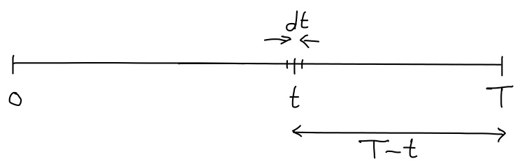
Figure Illustration of slicing the time interval $[0,T]$ into infinitesimally small time intervals of length $dt\text{.}$

The small quantity added during this infinitesimal time period $dt$ is "rate of renewal times time", or $R(t) \ dt.$
The length of the time interval $[t,T]$ is $T-t\text{.}$ Thus, the proportion of the small quantity added that survives/remains at time $T$ is $S(T-t).$
The amount of the small quantity that is added at time $t$ AND that survives/remains at time $T$ is the product of the above, that is, $dQ = S(T-t) \cdot R(t) \ dt.$
The total quantity that is added during the time period from $t=0$ to $t=T$ AND that survives/remains at time $T$ is $\int dQ = \int_0^T S(T-t) \cdot R(t) \ dt.$

🔗

Putting everything together, we have that

$Q(T)$ is the initial amount that survives/remains at time

$T$ PLUS the amount that has been added during the time interval

$[0,T]$ and survives/remains at time

$T\text{,}$ namely

$\begin{alignat*}{1} Q(T) &= S(T) \cdot Q(0) + \int dQ\\ &= S(T) \cdot Q(0) + \int_0^T S(T-t) \cdot R(t) \ dt. \end{alignat*}$

🔗

Checkpoint 6.2.6. Future Value from Survival and Renewal.

Consider a lake with trout. There currently are 5600 trout in the lake.

The trout are reproducing at the rate $\displaystyle R(t) = 720 e^{0.1t}$ trout/year. However, pollution is killing many of the trout; the proportion that survive after $t$ years is given by $\displaystyle S(t) = e^{-0.2t}\text{.}$

How many trout will be in the lake 10 years from now?

Solution

Let $P(t)$ be the number of trout in the lake at time $t\text{,}$ measured in years.

We are given $P(0) = 5600$ trout, and $T = 10$ years. Then

\begin{alignat*}{1} P(10) &= S(10) \cdot P(0) + \int_0^{10} S(10-t) \cdot R(t) \ dt \\ &= e^{-0.2(10)} \cdot 5600 + \int_0^{10} e^{-0.2(10-t)} \cdot 720 e^{0.1t} \ dt \\ &= 5600 e^{-2} + 720 \int_0^{10} e^{-2+0.2t+0.1t} \ dt \\ &= 5600 e^{-2} + 720 e^{-2} \int_0^{10} e^{0.3t} \ dt \\ &= 5600 e^{-2} + 720 e^{-2} \left. \left( \frac{ e^{0.3t} }{0.3} \right) \right|_0^{10} \\ &= 5600 e^{-2} + \frac{ 720 e^{-2} }{0.3} \left( e^{3} - 1 \right) \\ &= 5600 e^{-2} + 2400 \left( e - e^{-2} \right) \\ &\approx 6956.95. \end{alignat*}

Thus, we expect the number of trout in the lake 10 years from now to be about 6957.

Credit: J. Stewart and T. Day, Biocalculus: Calculus for the Life Sciences, 2015, Cengage Learning.

🔗

Subsection 6.2.3 Summary

🔗

Future Value from Net Change or Cumulative Change.

Suppose a quantity $Q$ changes over time at a known rate $Q'(t)\text{.}$
- The net (cumulative) change in Q between $t=a$ and $t=b$ is $Q(b) - Q(a) = \int_a^b Q'(t) \ dt.$
- The future value of $Q$ at time $T$ is $Q(T) = Q(0) + \int_0^T Q'(t) \ dt.$

🔗

Future Value from Survival and Renewal.

Suppose a quantity $Q(t)$ has initial value $Q(0)\text{,}$ renewal function $R(t)$ that represents the rate at which the quantity increases, and survival function $S(t)$ that represents the proportion of the quantity that survives/remains after $t$ years.
- The future value of $Q$ at time $T$ is $Q(T) = S(T) \cdot Q(0) + \int_0^T S(T-t) \cdot R(t) \ dt.$

🔗

Subsection 6.2.4 Don't Forget

🔗

Don't forget to return to eClass to complete the pre-class quiz.

🔗

Subsection 6.2.5 Further Study

🔗

Remember that the notes presented above only serve as an introduction to the topic. Further study of the topic will be required. This includes working through the pre-class quizzes, reviewing the lecture notes, and diligently working through the homework problems.

🔗

As you study, you should reflect on the following learning outcomes, and critically assess where you are on the path to achieving these learning outcomes:

🔗

Learning Outcomes

Recall and apply the formula to determine the future value of a quantity given its initial value and a rate of change.
Recall and apply the formula to determine the future value of a quantity given its initial value, the renewal function, and the survival function.

🔗

The following references provide a good start for review and further study:

Learning Outcome	Video	Textbook Section
1	N/A	5.3
2	N/A	6.3 (Examples 1, and Exercises 1 - 8)