Modelling with the "Rate In" - "Rate Out" Modelling Paradigm

Section 8.1 Modelling with the "Rate In" - "Rate Out" Modelling Paradigm

In this section, we focus on differential equations that arise from a consideration of a net rate of change of a quantity of interest. The quantity of interest may be

the size of a population (taking into account birth and death rates, or rates of immigration and emigration, for example)
the amount of drug in the body (taking into account administration or drug intake and elimination or breakdown of the drug),
the amount of a polluting chemical in a lake (taking into account inflow and outflow or removal),
the amount of carbon dioxide in the lungs (taking into account inhalation/ventilation, absorption, and excretion), etc.

🔗

The resulting differential equation is often autonomous, which means that we can use qualitative analysis (phase plot analysis) to gain insight about the behaviour of the quantity of interest. In some cases, we go a step further and obtain an explicit solution, that is, a function that gives the exact quantity of interest as a function of time.

🔗

In what follows, we review a couple of examples that we encountered previously.

🔗

Subsection 8.1.1 Intravenous Drug Dosing

🔗

Suppose that a drug is administered to a patient through an intravenous line at a rate of 8 mg/hr, and that the drug has a half-life of 24 hours.

🔗

Here, the quantity of interest is the amount of drug in the blood as a function of time. We let

$y(t)$ be the amount of the drug in the blood, measured in mg, at time

$t\text{,}$ measured in hours.

🔗

If we let

$R_{in}$ be the rate at which the amount of the drug increases, then we can write

$R_{in} = 8.$

🔗

We are given the half-life of the drug,

$T_{1/2} = 24\text{.}$ This implies that, in the absence of drug administration, the amount of drug decays exponentially with a rate constant of

$\lambda = \frac{ \ln(2) }{ T_{1/2} } = \frac{ \ln(2) }{ 24 }.$ If we let

$R_{out}$ be the rate at which the amount of the drug decreases, then we can write

$R_{out} = - \lambda y.$ where we are using the World's Most Important Differential Equation to model exponential decay. Putting these two rates together, the net rate of change is

$\begin{alignat*}{1} \frac{dy}{dt} &= R_{in} - R_{out} \\ &= 8 - \lambda y. \end{alignat*}$

🔗

Checkpoint 8.1.1.

Confirm that the units of each term in the differential equation are the same. What are the units of each term?

Solution

The units of $dy/dt$ are the units of $y$ divided by the units of $t\text{,}$ that is, mg/hr.
The units of $R_{in}$ are mg/hr (given).
The units of $\lambda$ are 1 divided by the units of $T_{1/2}\text{,}$ that is, 1/hr.
The units of $R_{in}$ are the units of $\lambda$ times the units of are $y\text{,}$ that is 1/hr times mg, or mg/hr.

In conclusion, the units of each term are the same, namely mg/hr.

🔗

We recognize the resulting differential equation as a separable differential equation for the unknown function

$y(t)\text{.}$ We leave it to the reader to determine

$y(t)\text{.}$

🔗

Checkpoint 8.1.2.

Determine the solution of the differential equation subject to the initial condition $y(0) = 0\text{.}$

Hint

Review the annotated lecture notes for Thursday of Week 7.

Answer

$y(t) = \frac{ 192 }{ \ln(2) } \left( 1 - e^{ -\frac{\ln(2)}{24} t }\right)\text{.}$

🔗

The amount of drug in the blood is at equilibrium when the rate at which the drug is administered balances the rate at which the body eliminates the drug, that is, when

$R_{in} = R_{out}\text{.}$

🔗

Subsection 8.1.2 Hormone Production and Removal

🔗

We consider

$H(t)\text{,}$ the amount of a certain hormone in the blood as a function of time

$t\text{.}$

🔗

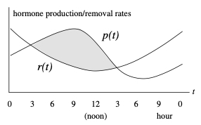
Suppose that the rate of hormone production as a function of time is

$R_{in} = p(t)\text{,}$ and the rate of deactivation of the hormone as a function of time is

$R_{out} = r(t)\text{,}$ then the net rate of change of

$H(t)$ is

$\begin{alignat*}{1} \frac{dH}{dt} &= R_{in} - R_{out} \\ &= p(t) - r(t). \end{alignat*}$

🔗

In class, we considered the situation where

$p(t)$ and

$q(t)$ are periodic functions, with a period of 24 hours, and with different phases, as illustrated below.

🔗
FigureGraph of the rate of hormone production, $p(t)\text{,}$ and the rate of hormone removal, $r(t)\text{.}$ Source: Integral Calculus with Applications to the Life Sciences, Leah Edelstein-Keshet, UBC, 2014.

🔗

Even though we do not know the dependence of

$p(t)$ and

$q(t)$ on

$t$ explicity, we can reason about the behaviour of

$H(t)$ over time. For example, we can conclude that

$H(t)$ increases between 3 AM and 3 PM, because

$p(t) \gt r(t)\text{,}$ that is,

$H'(t) \gt 0$ on this time interval. Similarly,

$H(t)$ decreases between 3 PM and 3 AM the next day, because

$p(t) \lt r(t)\text{,}$ that is,

$H'(t) \lt 0$ on this time interval. Thus, the amount of the hormone reaches a maximum at 3 PM, and a minimum at 3 AM.

🔗

Checkpoint 8.1.4.

Interpret the area of the shaded region in terms of the biological situation.

Answer

The area of the shaded region is $$ \int_{3}^{15} \left( p(t) - r(t) \right) \ dt = \int_{3}^{15} H'(t) \ dt, $$ which is the net increase of the amount of hormone between 3 AM and 3 PM.

🔗

Subsection 8.1.3 Summary

🔗

Differential equations often are set up with the "Rate In - Rate Out" modelling paradigm: $\frac{dy}{dt} = R_{in} - R_{out},$ where
- $R_{in}$ is the rate at which $y$ is produced, or the rate at which $y$ enters a compartment;
- $R_{out}$ is the rate at which $y$ is destroyed/broken down, or the rate at which $y$ leaves a compartment.

🔗

Subsection 8.1.4 Don't Forget

🔗

Don't forget to return to eClass to complete the pre-class quiz.

🔗

Subsection 8.1.5 Further Study

🔗

Remember that the notes presented above only serve as an introduction to the topic. Further study of the topic will be required. This includes working through the pre-class quizzes, reviewing the lecture notes, and diligently working through the homework problems.

🔗

As you study, you should reflect on the following learning outcomes, and critically assess where you are on the path to achieving these learning outcomes:

🔗

Learning Outcomes

Based on a narrative, interpret or set up a differential equation using the "Rate In - Rate Out" modelling paradigm.

🔗

The following references provide a good start for review and further study:

Learning Outcome	Video	Textbook Section
1	N/A	7.4 (Exercises 43, 45-48)