Phase Plane Analysis

Section 9.2 Phase Plane Analysis

In this section, we develop tools to perform phase plane analysis, which is to obtain a qualitative understanding of the nature of the solutions of a system of two autonomous differential equations. Conceptually, phase plane analysis is an extension of a phase plot analysis for a single autonomous differential equation into the two-dimensional phase plane.

🔗

Subsection 9.2.1 Equilibria

🔗

Consider the following system of two autonomous differential equations:

$\begin{alignat*}{1} \frac{dx}{dt} &= f(x,y) \\ \frac{dy}{dt} &= g(x,y). \end{alignat*}$

🔗

An equilibrium is a pair of values

$(\hat{x},\hat{y})$ such that both

$\displaystyle \frac{dx}{dt} = 0$ and

$\displaystyle \frac{dy}{dt} = 0$ when

$x=\hat{x}$ and

$y = \hat{y}\text{,}$ that is, when

$f(\hat{x},\hat{y}) = 0$ and

$g(\hat{x},\hat{y}) = 0$ simultaneously.

🔗

Example 9.2.1.

Find the equilibria of the system

\begin{alignat*}{1} \frac{dx}{dt} &= x(3-x-y) \\ \frac{dy}{dt} &= y(2-x-y). \end{alignat*}

for $x,y \ge 0\text{.}$

Solution

$\displaystyle \frac{dx}{dt} = 0$ when $x(3-x-y) = 0\text{,}$ that is, when

1.: $x=0\text{,}$ or
2.: $y=3-x\text{.}$

Similarly, $\displaystyle \frac{dy}{dt} = 0$ when $y(2-x-y) = 0\text{,}$ that is, when

3.: $y=0\text{,}$ or
4.: $y=2-x\text{.}$

Combining conditions 1 and 3:

This gives the equilibrium $(\hat{x},\hat{y}) = (0,0)\text{.}$

Combining conditions 1 and 4:

Substituting $x=0$ into $y=2-x$ gives $y=2\text{,}$ resulting in the equilibrium $(\hat{x},\hat{y}) = (0,2)\text{.}$

Combining conditions 2 and 3:

Substituting $y=0$ into $y=3-x$ gives $x=3\text{,}$ resulting in the equilibrium $(\hat{x},\hat{y}) = (3,0)\text{.}$

Combining conditions 2 and 4:

$y$ cannot simultaneously be equal to $3-x$ and $2-x\text{.}$ Therefore there is no equilibrium point resulting from combining conditions 2 and 4.

In summary, the given system of differential equations has three equilibria, namely $(0,0)\text{,}$ $(0,2)\text{,}$ and $(3,0)\text{.}$

🔗

Subsection 9.2.2 Nullclines

🔗

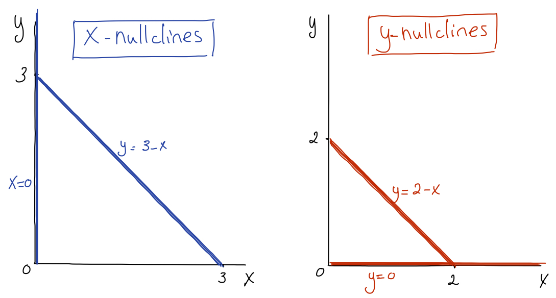
Referring to the previous example, the curves

$x=0$ and

$y=3-x$ are the curves in the

$(x,y)$ plane where

$\displaystyle \frac{dx}{dt} = 0\text{.}$ We call these curves the

$x$ -nullclines of the given system of differential equations. Similarly, the curves

$y=0$ and

$y=2-x$ are the curves where

$\displaystyle \frac{dy}{dt} = 0\text{,}$ and they are called the

$y$ -nullclines.

🔗

The following figure shows the nullclines. For ease of recognition throughout,

$x$ -nullclines will be drawn in blue, and

$y$ -nullclines will be drawn in red.

🔗
Figure 9.2.2. Visualization of the nullclines for our example.

🔗

In general, the

$x$ -nullclines of the system of differential equations

$\begin{alignat*}{1} \frac{dx}{dt} &= f(x,y) \\ \frac{dy}{dt} &= g(x,y) \end{alignat*}$

🔗

are the curves in the

$(x,y)$ phase plane that satisfy the equation

$f(x,y)=0\text{.}$ Along these curves,

$\displaystyle \frac{dx}{dt} = 0\text{.}$ Similarly, the

$y$ -nullclines of the system of differential equations are the curves in the

$(x,y)$ phase plane that satisfy the equation

$g(x,y)=0\text{.}$ Along these curves,

$\displaystyle \frac{dy}{dt} = 0\text{.}$

🔗

Subsection 9.2.3 Finding Equilibria Graphically

🔗

Any point at which an

$x$ -nullcline intersects a

$y$ -nullcline is an equilibrium. In the following figure, we show the superposition of the two sets of nullclines in the phase plane, and indicate the equilibria with black dots.

🔗
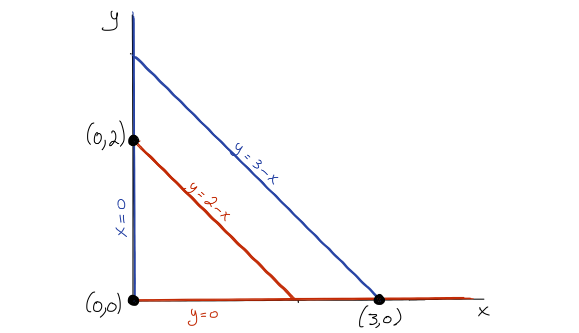
Figure 9.2.3. Visualization of the equilibria for our example.

🔗

Remark 9.2.4.

Equilibria are found only at the intersection of a blue curve and a red curve!

🔗

Subsection 9.2.4 Qualitative Dynamics in the Phase Plane

🔗

The

$x$ -nullclines separate regions where either

$\displaystyle \frac{dx}{dt} \gt 0$ (that is, where

$x$ is increasing) or

$\displaystyle \frac{dx}{dt} \lt 0$ (that is, where

$x$ is decreasing).

🔗

Similarly,

$y$ -nullclines separate regions where either

$\displaystyle \frac{dy}{dt} \gt 0$ (that is, where

$y$ is increasing) or

$\displaystyle \frac{dy}{dt} \lt 0$ (that is, where

$y$ is decreasing).

🔗

In the following figure, we use horizontal arrows to indicate the regions where

$x$ is increasing (right-pointing arrows) or decreasing (left-pointing arrows), and vertical arrows to indicate the regions where

$y$ is increasing (upward-pointing arrows) or decreasing (downward-pointing arrows).

🔗
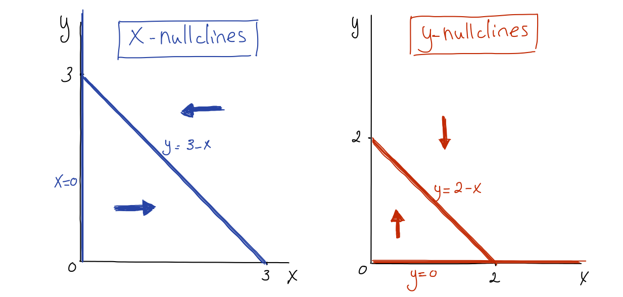
Figure 9.2.5. Visualization of the horizontal and vertical direction arrows in various regions of the phase plane for our example.

🔗

To determine the direction of a horizontal arrow in a particular region, choose a test point inside that region, and determine whether

$\displaystyle \frac{dx}{dt} = f(x,y) \lt 0$ or

$\gt 0\text{.}$ For example, in the figure on the left, the point

$(1,1)$ lies below the

$x$ -nullcline

$y=3-x\text{.}$ We evaluate

$f(1,1) = 1 (3-1-1) \gt 0\text{,}$ therefore

$x$ is increasing in the region below the

$x$ -nullcline

$y=3-x\text{,}$ and the horizontal arrow below this nullcline is pointing to the right.

🔗

Similarly, to determine the direction of a vertical arrow in a particular region, choose a test point inside that region, and determine whether

$\displaystyle \frac{dy}{dt} = g(x,y) \gt 0$ (resulting in an upward-pointing arrow) or

$\lt 0$ (resulting in a downward-pointing arrow).

🔗

Superimposing the nullclines and arrows results in the following figure, where the black arrows give the overall direction of movement of a solution trajectory.

🔗
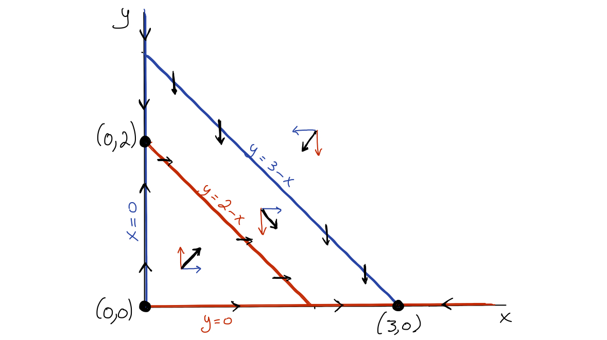
Figure 9.2.6. Visualization of the direction arrows in all regions of the phase plane for our example.

🔗

Remark 9.2.7.

On any

$x$ -nullcline,

$x$ does not change, and the movement is purely vertical. Similarly, on any

$y$ -nullcline,

$y$ does not change, and the movement is purely horizontal.

🔗

Following the general direction of the arrows, we can infer solution trajectories from several initial conditions, as shown in the figure below (the solution trajectories are sketched in green).

🔗
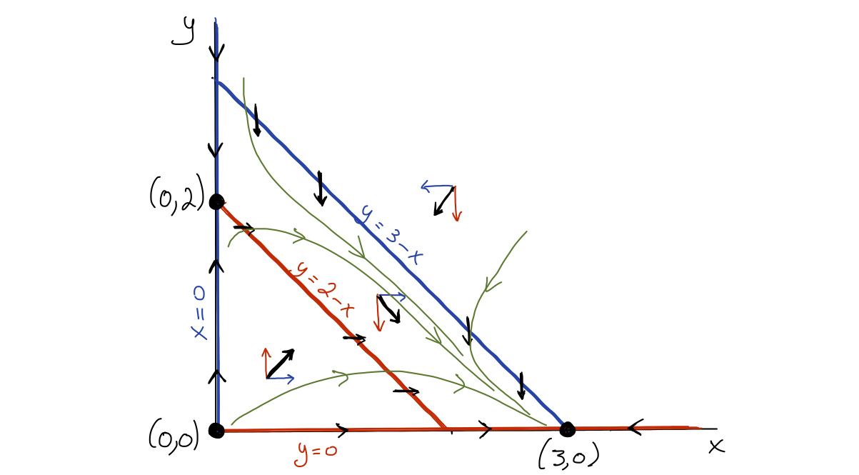
Figure 9.2.8. Visualization of the qualitative nature of solutions in the phase plane for our example.

🔗

It appears that most initial conditions result in a solution that eventually ends up at

$(3,0)\text{.}$ We therefore expect the equilibrium

$(3,0)$ to be locally stable, and both

$(0,0)$ and

$(0,2)$ to be unstable.

🔗

Any initial condition

$(0,y_0)$ for

$y_0 > 0$ results in a solution that eventually ends up at

$(0,2)\text{.}$ However, for any small deviation to the right off the

$y$ -axis, the solution ends up at

$(3,0)$ instead.

🔗

Subsection 9.2.5 An Online Tool for Qualitative Dynamics in the Phase Plane

🔗

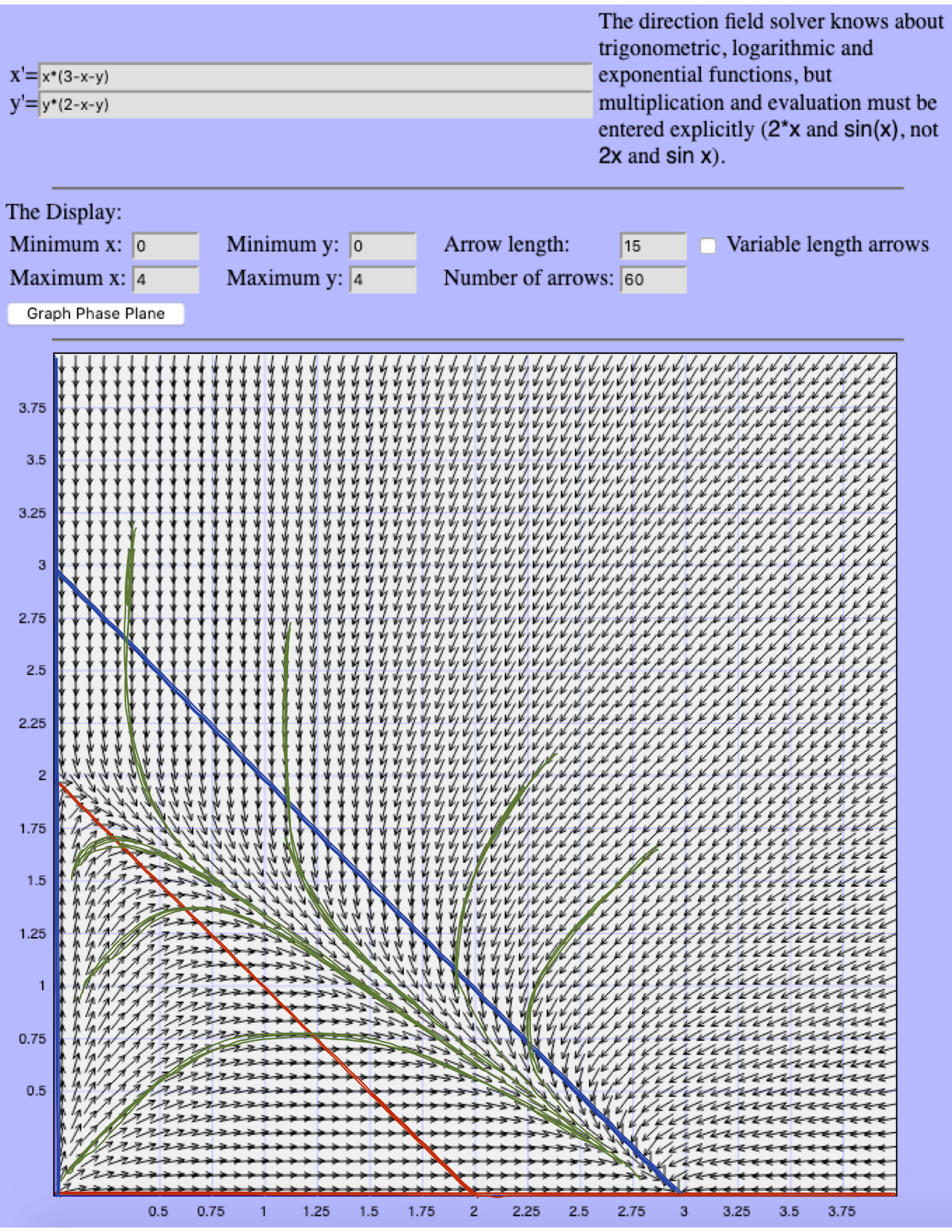
Ariel Barton at the University of Arkansas has created a basic but functional tool to draw many directional arrows in the phase plane for a given set of differential equations in the form

$\begin{alignat*}{1} \frac{dx}{dt} &= f(x,y) \\ \frac{dy}{dt} &= g(x,y). \end{alignat*}$

🔗

The tool can be found at https://aeb019.hosted.uark.edu/pplane.html.

🔗

It is possible to choose the number of direction arrows. For example, setting "Number of arrows" to 20 results in 20 arrows across as well as 20 arrows down (for a total of 400 direction arrows). The more arrows, the easier it is to infer the flow of the solutions.

🔗

The following figure is a screenshot of the phase plane generated for our example, with the nullclines and some solutions drawn in.

🔗
Figure 9.2.9. Screenshot from https://aeb019.hosted.uark.edu/pplane.html for our example, with the nullclines and representative solutions drawn in.

🔗

Subsection 9.2.6 Caution

🔗

While we were able to infer the stability of the equilibria for the system of differential equations in our example, it is often not possible from the direction arrows.

🔗

Particularly tricky are situations where there appears to be circular motion around an equilibrium, such as shown in the following figure.

🔗
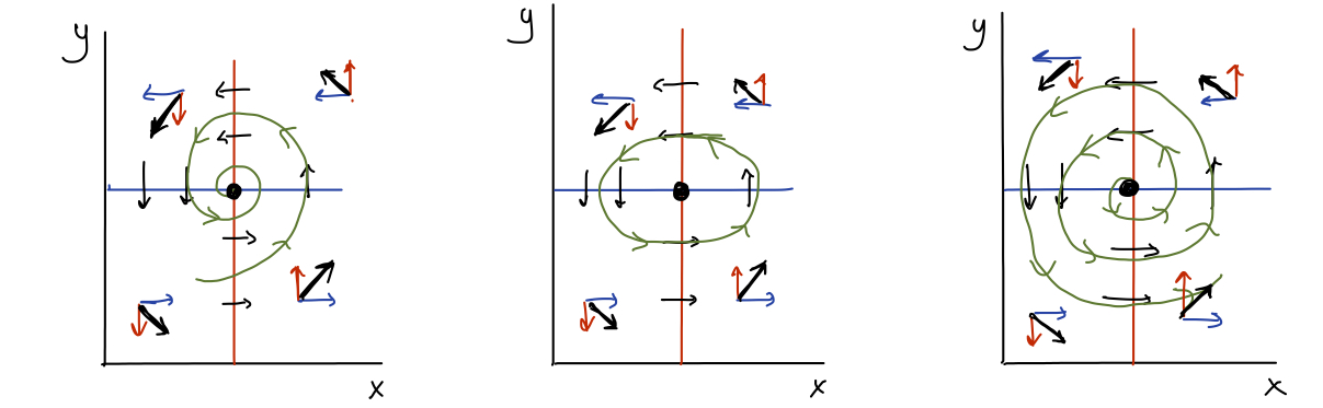
Figure 9.2.10. Visualization of three solution types that are consistent with circular motion in the phase plane.

🔗

Remark 9.2.11.

Note that there may be a periodic solution around the equilibrium (as shown in the middle), or the solution could spiral in towards the equilibrium (as shown on the left), or out from the equilibrium (as shown on the right). The equilibrium in the figure on the left is locally stable, while the equilibrium in the figure on the right is unstable. The equilibrium in the middle figure is neither (it is a degenerate case, referred to as neutrally stable).

🔗

Determining the stability of equilibria in general is beyond the scope of MATH 136 (this requires techniques from Linear Algebra, and is treated in a course of ordinary differential equations [MATH 334] and courses on mathematical modelling [MATH 371 and 372])

🔗

Subsection 9.2.7 Summary

🔗

For the following system of two autonomous differential equations:

$\begin{alignat*}{1} \frac{dx}{dt} &= f(x,y) \\ \frac{dy}{dt} &= g(x,y) \end{alignat*}$
- An equilibrium of the system is a pair of values $(\hat{x},\hat{y})$ such that both $\displaystyle \frac{dx}{dt} = 0$ and $\displaystyle \frac{dy}{dt} = 0$ when $x=\hat{x}$ and $y = \hat{y}\text{,}$ that is, when $f(\hat{x},\hat{y}) = 0$ and $g(\hat{x},\hat{y}) = 0$ simultaneously.
- The $x$ -nullclines of the system are the curves in the $(x,y)$ phase plane that satisfy the equation $f(x,y)=0\text{.}$
  - On the $x$ -nullclines, $\displaystyle \frac{dx}{dt} = 0\text{.}$
  - The $x$ -nullclines separate regions where either $\displaystyle \frac{dx}{dt} \gt 0$ (that is, where $x$ is increasing) or $\displaystyle \frac{dx}{dt} \lt 0$ (that is, where $x$ is decreasing).
- The $y$ -nullclines are the curves in the $(x,y)$ phase plane that satisfy the equation $g(x,y)=0\text{.}$
  - On the $y$ -nullclines, $\displaystyle \frac{dy}{dt} = 0\text{.}$
  - The $y$ -nullclines separate regions where either $\displaystyle \frac{dy}{dt} \gt 0$ (that is, where $y$ is increasing) or $\displaystyle \frac{dy}{dt} \lt 0$ (that is, where $y$ is decreasing).
- Any intersection of an $x$ -nullcline and a $y$ -nullcline is an equilibrium.

🔗

Subsection 9.2.8 Don't Forget

🔗

Don't forget to return to eClass to complete the pre-class quiz.

🔗

Subsection 9.2.9 Further Study

🔗

Remember that the notes presented above only serve as an introduction to the topic. Further study of the topic will be required. This includes working through the pre-class quizzes, reviewing the lecture notes, and diligently working through the homework problems.

🔗

As you study, you should reflect on the following learning outcomes, and critically assess where you are on the path to achieving these learning outcomes:

🔗

Learning Outcomes

Determine the nullclines of a system of two autonomous differential equations.
Determine the equilibria of a system of two autonomous differential equations algebraically and graphically.
Use phase plane analysis to determine the qualitative nature of the solutions of a system of two autonomous differential equations.
For a system of two autonomous differential equations that represents the predator-prey relationship between two species, identify which of the variables represents the predator population and which represents the prey population.

🔗

The following references provide a good start for review and further study:

Learning Outcome	Video	Textbook Section
1	N/A	7.6
2	N/A	7.6
3	N/A	7.6
4	N/A	7.5 and 7.6