Section 11.2 Functions of Several Variables
By now, we are very familiar with the calculus of single-variable functions such as \(y = f(x)\) such as \(y = 1 - x\text{,}\) \(y = x^2\text{,}\) and \(y = \sin(x)\text{.}\)
In this section, we begin the study of multi-variable functions. Mathematically, we are interested in a function of two variables, for example \(z = f(x, y) = \sin(x+y)\text{,}\) or in a function of three variables, for example \(f(x, y, z) = x^2 + y^2 + z^2\text{,}\) or more generally in a function of \(n\) variables, \(f( x_1, x_2, \ldots, x_n )\text{.}\)
Subsection 11.2.1 Visualizing Functions of Two Variables: Surfaces and Contour Plots
Formally, a function of two variables, \(f\text{,}\) is a rule that assigns to each point \((x,y)\) in the domain \(D\) a real number \(z = f(x,y)\text{.}\) Functions of two variables define surfaces in \(\mathbb{R}^3\) which we often can visualize.
If \(f\) is a function of two independent variables with domain \(D\text{,}\) then the graph of \(f\) is the set of all points \((x,y,z)\) such that \(z = f(x,y)\) for all \((x,y)\) in \(D\text{.}\)
Note that we now work with coordinate triplets, \((x,y,z)\text{.}\) We locate each point \((x,y,z)\) in \(\mathbb{R}^3\) using the Cartesian coordinate system. An example of a surface visualized in \(\mathbb{R}^3\) is the blue shape in the left figure below:
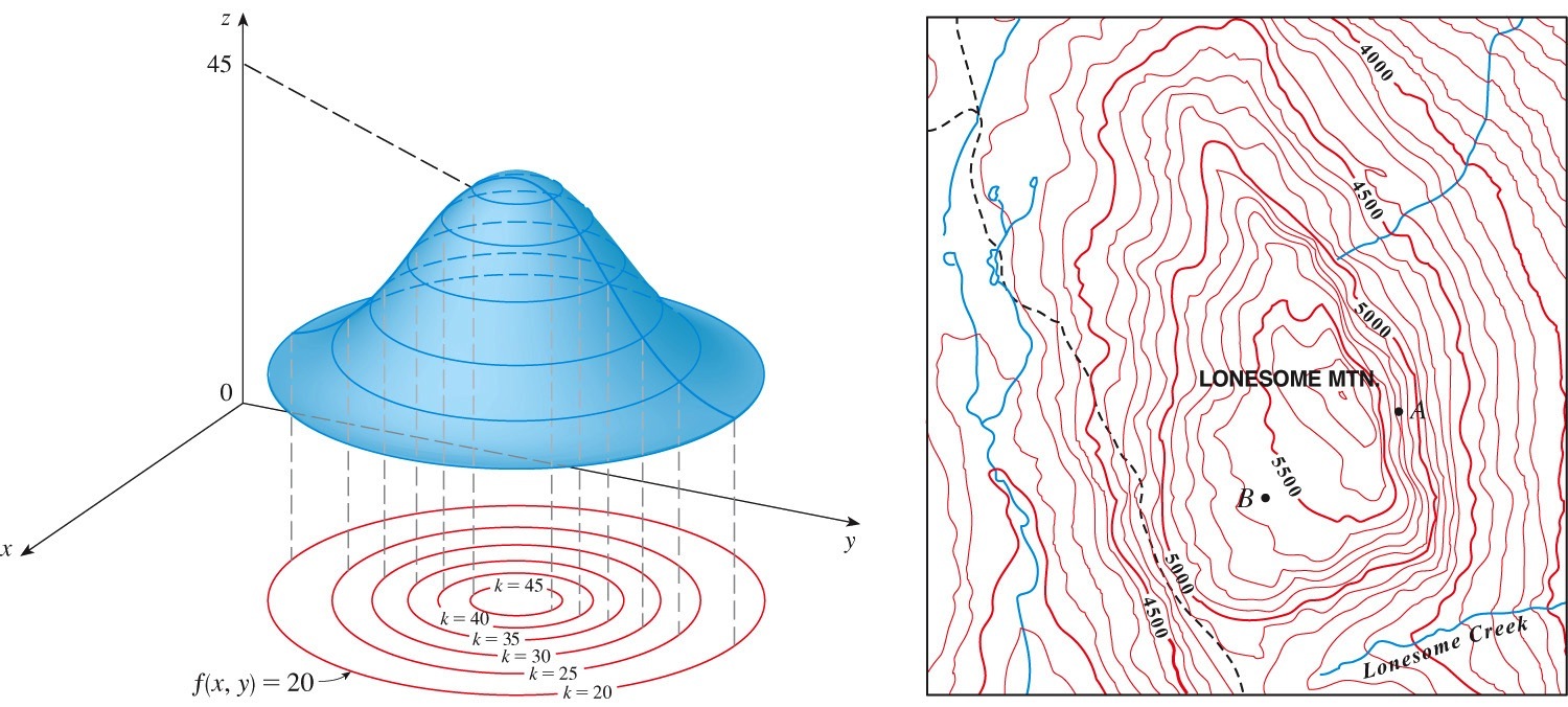
A complementary method to visualize functions of two variables is the contour plot. A contour plot is like a topographical map showing the level curves (see the right figure above).
A level curve of \(z=f(x,y)\) consists of the points \((x,y)\) in the \(xy\) plane with equations \(f(x,y)=k\text{,}\) where \(k\) is a constant in the range of \(f\text{.}\)
In the left figure above, the level curves of the surface \(z=f(x,y)\) are projected onto the \(xy\) plane.
In what follows, we present two specific examples. For each example, we show the surface in \(\mathbb{R}^3\) on the left, and level curves in the corresponding contour plot immediately to the right.
Subsection 11.2.2 Visualization of a Function of Two Variables (Example 1)
Consider $$ z= f(x,y) = x^2 + y^2. $$ The surface and the corresponding contour plot are shown below.
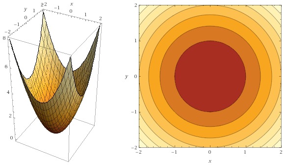
plot x^2 + y^2, x=-2..2 y=-2..2.To connect the equation of the surface, \(z=f(x,y)=x^2+y^2\text{,}\) to its visualizations, recall that \(x^2 + y^2 = R^2\) is the equation of a circle with radius \(R\) centered at the origin in the \(xy\) plane. Therefore, each level curve given by \(x^2 + y^2 = k\) is a circle with radius \(\sqrt{k}\) centered at the origin in the \(xy\) plane. Equivalently, the intersection of the horizontal plane \(z=k\) (any plane that is parallel to the \(xy\) plane) and the surface is a circle with radius \(\sqrt{k}\text{.}\) The larger the value of \(k\text{,}\) the larger the circle.
The circles are clearly shown in the contour plot. Here, seven level curves \(x^2 + y^2 = k\) are shown, for \(k=1, 2, \ldots, 7\text{.}\) The level curve given by \(k=4\) is a circle of radius \(2\) in the \(xy\) plane.
Checkpoint 11.2.3.
The surface is called a paraboloid. Note that the intersection of the surface with the \(yz\) plane (defined by \(x=0\)) is the parabola \(z = y^2\text{.}\) Similarly, the intersection of the surface with the \(xz\) plane (defined by \(y=0\)) is the parabola \(z=x^2\text{.}\)
Checkpoint 11.2.4.
Subsection 11.2.3 Visualization of a Function of Two Variables (Example 2)
Consider $$ z= f(x,y) = 1 + y^2. $$ The surface and the corresponding contour plot are shown below.
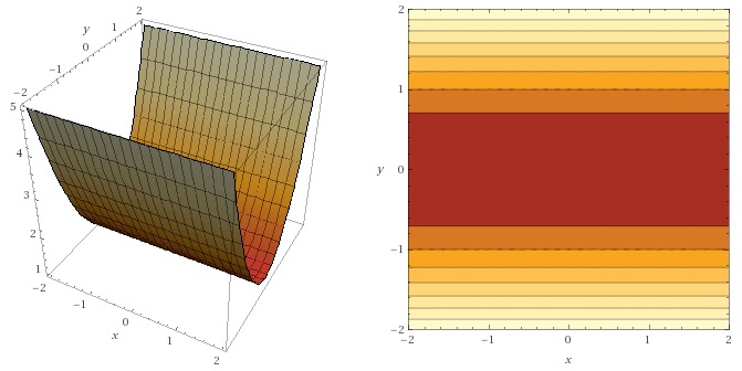
plot3d 1 + y^2, x=-2..2 y=-2..2.To connect the equation of the surface, \(z=f(x,y)=1+y^2\text{,}\) to its visualizations, note that is independent of the value of \(x\text{.}\) That is, the intersection of each vertical plane \(x=c\) (any plane parallel to the \(yz\) plane) with the surface is the parabola \(z=1+y^2\text{.}\)
The parabolic shape can be seen clearly in the plot in \(\mathbb{R}^3\text{.}\)
The level curves are \(1 + y^2 = k\text{,}\) that is \(y = \sqrt{k-1}\text{,}\) which are horizontal lines (as expected, since the surface is independent of \(x\)), as seen in the contour plot.
Subsection 11.2.4 More Practice (Optional)
Checkpoint 11.2.6.
plot sin( sqrt( x^2 + y^2 ) ).Checkpoint 11.2.7.
plot 6 - 3x - 2y.Checkpoint 11.2.8.
plot abs(x) + abs(y).Checkpoint 11.2.9.
plot abs(xy).Checkpoint 11.2.10.
plot 1 / ( 1 + x^2 + y^2 ), x=-2..2 y=-2..2.Checkpoint 11.2.11.
plot ( x^2 - y^2 )^2, x=-3..3 y=-3..3.Checkpoint 11.2.12.
plot ( x - y )^2, x=-3..3 y=-3..3.Checkpoint 11.2.13.
plot sin( abs(x) + abs(y) ), x=-6..6 y=-6..6.Subsection 11.2.5 Visualizing Functions of Three or More Variables
Unfortunately, we are not able to visualize functions of three or more variables very easily, as we would need to visualize in \(\mathbb{R}^4\) or higher-dimensional space. To gain insight into how these functions behave, one might think about the behaviour on certain convenient cross-sections by setting one or more variables equal to a constant (similar to what we did in the previous section, for example by considering the intersection of the horizontal plane \(z=k\) with the surface). This is not easy though, and certainly not a learning outcome for this course.
Subsection 11.2.6 Summary
- If \(f\) is a function of two independent variables with domain \(D\text{,}\) then the graph of \(f\) is the set of all points \((x,y,z)\) such that \(z = f(x,y)\) for all \((x,y)\) in \(D\text{.}\)
- A level curve of \(z=f(x,y)\) consists of the points \((x,y)\) in the \(xy\) plane with equations \(f(x,y)=k\text{,}\) where \(k\) is a constant in the range of \(f\text{.}\)
- A contour plot is a graph in the \(xy\) plane with a set of level curves of \(z=f(x,y)\text{.}\)
Subsection 11.2.7 Don't Forget
Don't forget to return to eClass to complete the pre-class quiz.
Subsection 11.2.8 Further Study
Remember that the notes presented above only serve as an introduction to the topic. Further study of the topic will be required. This includes working through the pre-class quizzes, reviewing the lecture notes, and diligently working through the homework problems.
As you study, you should reflect on the following learning outcomes, and critically assess where you are on the path to achieving these learning outcomes:
Learning Outcomes
- Use technology to generate a graph of the surface for a given function of two variables and the corresponding contour plot.
- Describe the relationship between a graph of the surface for a given function of two variables and the level curves in the corresponding contour plot.
The following references provide a good start for review and further study:
| Learning Outcome | Video | Textbook Section |
|---|---|---|
| 1 | N/A | 9.1 |
| 2 | N/A | 9.1 |