An Example With Different Complexity Classes#
Sometimes we can improve an algorithm to the point where the run-time is in a different class of functions altogether. This kind of improvement is considered substantial and important. For example, suppose we have one algorithm that runs in linear time and another that runs in logarithmic time, for the same problem. The logarithmic algorithm is superior as we can see when we compare the graphs of the two:
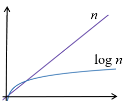
When \(n\) gets big, i.e. \(n\) approaches infinity, there will be a point where the logarithmic algorithm is always faster than the linear one, no matter what constants may be part of the run-time complexity of either function. In other words, the linear function grows faster than the logarithmic function, which means that for sufficiently large \(n\), the algorithm running at linear time will take substantially longer than the one running at logarithmic time.
Sequential Search Complexity#
A common task done by computers is to search for someone’s record. The record typically has an id number (called a key associated with it, and all records for a company might be stored in a list (perhaps an array). The search process must find the required record from the list. One algorithm to do this is sequential search. Here is the algorithm in Java, where we simply want to find the index of whatToFind in theList:
1.  public static int sequentialSearch(int whatToFind, int[] theList){
2.     for (int i = 0; i < theList.length; i++){
3.        if (whatToFind == theList[i]){
4.           return i;
5.        }
6.     }
7.   return -1; //not found
8.  }
If we attempt to find the run-time complexity, we soon realize that it will vary depending on where the item is located, or not located, in the list. Suppose we are working on this list:
[4, 5, 9, 14, 84, 32, 3, 12]
Let us count the key comparisons, that is the comparisons to the id number in the code: whatToFind == theList[i] in line 3. Check how many key comparisons to find each of the items and also items not in the list.
|
Number of Key Comparisons |
|---|---|
4 |
1 |
5 |
2 |
9 |
3 |
14 |
4 |
84 |
5 |
32 |
6 |
3 |
7 |
12 |
8 |
Item not in list |
8 |
We rarely care about the best search time, when the item we want is right at the beginning but we do care about the worst search time, and later with more computing knowledge, the average search time. The worst time occurs when we are looking for the last item, or when the item is not in our list. In both of these cases, we must look at everything in the list. Specifically, if we count key comparisons, then on a list of size \(n\), our worst case will be \(n\) key comparisons. We conclude that the worst-case run-time of sequential search is \(θ(n)\) or linear.
This begs the question of whether we can write a better search algorithm. And what does better look like? We have already seen that better than linear is logarithmic (constant time is even better, and surprisingly it could be achieved as we will see in later courses). Let’s aim for logarithmic time.
Binary Search Complexity#
Logarithmic implies making the problem significantly smaller each time, for example cutting the problem space in half each time. Consider searching for a word in an old-fashioned paper dictionary. We do not go along looking at every single entry for the word of which we want the definition. Rather, we quickly move closer, based on the sorting of the words in the dictionary. An algorithm similar to this dictionary look-up is called binary search, and it works only if the list is sorted.
Binary Search is shown here in Java:
1.  public static int binarySearch(int whatToFind, int[] theList){
2.     int low = 0;
3.     int high = theList.length - 1;

4.     while(high >= low){
5.        int middle = (low + high) / 2;

6.        if (theList[middle] == whatToFind){
7.           return middle;
8.        }

9.        if (theList[middle] < whatToFind){
10.          low = middle + 1;
11.       }
12.       else {
13.          high = middle - 1;
14.       }
15.    }//while

16.    return -1; //not found
17. }
Now let us determine the complexity of binary search by counting the key comparisons, as highlighted in the code. As in sequential search, we can see that the run-time will vary depending on the location of the item to be found. But will the worst case be as bad?
Consider the list:
[12, 17, 23, 25, 34, 39, 41, 50, 55, 59, 68]
How many key comparisons to find each of the numbers? Consider looking for 12, low starts at 0 and high at 10. middle is then 5, and the first place we check is the 39. 39 is clearly greater than 12, so with two key comparisons (== on line 6 and < on line 9) we know that high should become 5 – 1 = 4 and we continue with the loop. Now middle is 2 and the second place we check is the 23. Again two key comparisons send us to knowing we still need to look further left and high becomes 2 – 1 = 1. Now middle is 0 and we find the 12 with one key comparison. We build a table with the number of key comparisons to find each possible element:
|
. 
|
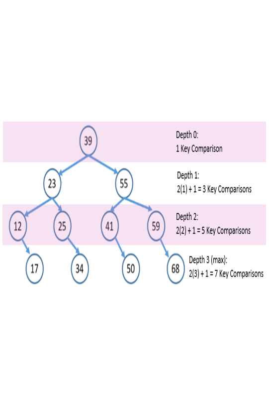
We could picture the search as a binary search tree, as shown on the right. Each element of the tree has a maximum depth of
where \(n\) is the size of the list[1]. The number of key comparisons depends on the depth of the item, but in the worst case it is
which puts the algorithm’s run-time into the set \(θ(\log n)\). This is a faster run-time than sequential search.
In summary, the run-time of binary search gives a complexity class improvement, considered a significant improvement from \(θ(n)\) to \(θ(\log n)\), over the run-time of sequential search. The catch, however, is that the list must be sorted before binary search would give a correct result. The programmer must beware. The complexity of sorting a list is fairly high, but lists can often be sorted while the users are sleeping, and then binary search can be used when speed matters.
Can’t Usually Have Your Cake and Eat it Too!
A faster run-time sometimes means an increased cost somewhere else. In binary search we get a faster run-time at the cost of needing the list to be sorted. This cost is in \(\theta (n^2)\) if running a simple sort or in \(\theta (n \log n)\) if running a more sophisticated sort. The good thing is that this sort can be run sometime before we need to search, for example, while we are sleeping.
Practice Questions#
Write Java code to find the maximum item, given any list of integers.
What is the run-time complexity of your code, counting key comparisons, from question 1? Find the complexity exactly and use order notation to describe it.
Assuming that you have a sorted list, from small to large, write Java code for finding the maximum key in the list. Ensure that your code runs in the fastest time possible.
What is the run-time complexity for your algorithm in question 3? Use order notation to describe the complexity.
How can you be sure that your algorithm is running in the fastest time possible?