Consider Rutherford scattering of an electron from a fixed Coulomb potential (figure 7.2).
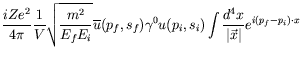
The ![]() -matrix is
-matrix is
| (7.26) |
In lowest order the wavefunctions reduce to plane waves:
| (7.27) | |||
| (7.28) |
where we have normalized to unit probability in a box of volume ![]() .
.
The Coulomb potential is
| (7.29) |
We are working in the Heaviside-Lorentz (rationalized Gaussian) system
of units.
If we were working in the Gaussian system of units, the Coulomb
potential would be
![]() .
Thus
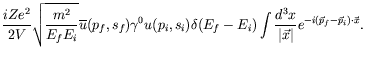
.
Thus
The space integral is the Fourier transform of the Coulomb potential
| (7.31) |
where
![]() .
Therefore
.
Therefore
| (7.32) |
The number of final states in the momentum interval ![]() is
is
![]() .
To see this we notice that standing waves in a cubic box of volume
.
To see this we notice that standing waves in a cubic box of volume
![]() require
require
| (7.33) |
with integer numbers ![]() .
For large
.
For large ![]() the descrete set of
the descrete set of ![]() -values approaches a
continum.
The number of states is (setting
-values approaches a
continum.
The number of states is (setting ![]() )
)
| (7.34) |
The transition probability per particle into these states is
| (7.35) |
The square of the ![]() -function is mathematically not well
defined, it is a divergent quantity and has to be specified by a
limiting procedure.
We can reason it to be
-function is mathematically not well
defined, it is a divergent quantity and has to be specified by a
limiting procedure.
We can reason it to be
| (7.36) |
If ![]() , as required by the other remaining delta function, then
, as required by the other remaining delta function, then
| (7.37) |
For ![]() ,
,
| (7.38) |
and
| (7.39) |
Another way of viewing this is that the finite time interval smears the delta-function
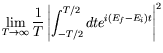 |
![$\displaystyle \lim_{T\rightarrow\infty} \frac{1}{T}
\left[ \frac{\sin(E_f-E_i)T/2}{(E_f-E_i)/2} \right]^2 ,$](img3138.png) |
||
| (7.40) |
Using wave-packets instead of plane waves removes the need to square the delta-function.
If we consider transitions in a time ![]() and divide out the time, we
obtain the rate, which is the number
and divide out the time, we
obtain the rate, which is the number ![]() of transitions per unit time
into momentum interval
of transitions per unit time
into momentum interval ![]() :
:
| (7.41) |
A cross-section is defined as the transition rate ![]() divided by the
flux of incident particles
divided by the
flux of incident particles
![]() , where
, where ![]() denotes the vector
component along the incident velocity
denotes the vector
component along the incident velocity
![]() .
With the normalization we have adapted, the flux is
.
With the normalization we have adapted, the flux is
| (7.42) |
Thus the differential cross-section, ![]() , per unit solid angle,
, per unit solid angle,
![]() , is
, is
| (7.43) |
Since
![]() , we obtain
, we obtain
which is the Rutherford scattering cross-section in the non-relativistic limit.
In general, one does not know the initial polarizations so we average over these. Also, one does not observe the final polarization so we sum over these.
It is important to note that this is an incoherent average, in the sense that we average the cross-section, rather than the amplitude.
Consider the spin sum
We remember
| (7.47) |
and notice that operating with ![]() , we have
, we have
| (7.48) |
The spin sum (eqaution 7.46) thus becomes
| (7.49) |
which is a trace. Therefore
Using trace theorems we have
| (7.51) |
and
| (7.52) |
The differential cross-section can be written in terms of the
scattering energy, ![]() , and scattering angle,
, and scattering angle, ![]() .
Since
.
Since ![]() ,
,
![]() , but
, but
![]() .
The kinematical relations become
.
The kinematical relations become
| (7.53) |
and
| (7.54) |
We find
| (7.55) |
This is the Mott cross-section.
It reduces to the Rutherford formula as
![]() .
Which agrees with the non-relativistic Born approximation for the
scattering amplitude
.
Which agrees with the non-relativistic Born approximation for the
scattering amplitude
| (7.56) |
![\begin{figure}\begin{center}
\begin{picture}(60,100)(0,0)
\SetWidth{0.75}
% Line...
...
\Text(35,80)[l]{$p_f,s_f$}
\end{picture}}
\end{picture}\end{center}\end{figure}](img3085.png)