Lifetimes and Cross-Sections

The $S$-matrix permits the calculation of two types of observable quantities, lifetimes and cross-sections. Both can be calculated from the transition probability per unit space-time volume. If there were no interaction between the particles, the state of the system would be unchanged, corresponding to a unit $S$-matrix (absence of scattering). It is convenient to separate this unit matrix in all cases, writing the scattering matrix in the form

$$S_{fi} = \delta_{fi} + R_{fi} ,$$

$$= \delta_{fi} + i (2\pi)^4 \delta^4 (p_f-p_i) T_{fi} ,$$ (7.1)

where $T_{fi}$ is another matrix. In the second term we have written separately the four-dimensional Dirac delta-function which comes from the integral

$$\frac{1}{(2\pi)^4} \int e^{i(p_f-p_i)\cdot x} d^4x = \delta^4(p_f-p_i) .$$ (7.2)

The Dirac delta-function expresses the law of conservation of four-momentum ($p_f$ and $p_i$ being the sums of the four-momentum of all the particles in the final and initial states), the other factors are included for subsequent convenience.

If one of the colliding particles is sufficiently heavy (and its state is unaltered by the collision) it acts only as a fixed source of a constant field in which the other particle is scattered. Since the energy (though not the momentum) of the system is conserved in a constant field, in this treatment of the collision process we can write the $S$-matrix elements in the form

$$S_{fi} = \delta_{fi} + i(2\pi)\delta(E_f-E_i)T_{fi} .$$ (7.3)

The structure of the scattering amplitude $T_{fi}$ is of the form

$$T_{fi} = u_1^* u_2^* \cdots Q \cdots u_2 u_1 ,$$ (7.4)

where on the left we have the amplitude of wave functions of final particles, and on the right those of initial particles; $Q$ is some matrix relating the indices of the wave amplitude components of all the particles.

Consider the transition of a system from an initial state $w_i$ to a final state $w_f\ne w_i$. The matrix element of $S$ may then be replaced by that of

$$R = S - I.$$ (7.5)

$$S_{fi} \equiv (w_f,Sw_i) = (f\vert S\vert i) = (f\vert R\vert i), \quad \mathrm{if} \quad w_f\ne w_i.$$ (7.6)

In momentum space the matrix elements of the operator $R$ are of the form

$$(f\vert R\vert i) = i(2\pi)^4\delta^4(p_f-p_i)(f\vert T\vert i) ,$$ (7.7)

where $p_i$ and $p_f$ are the initial and final four-momentum of the system. $(f\vert R\vert i)$ is the transition probability amplitude for a transition taking place over all space and all time from the infinite past to the infinite future. The corresponding transition probabability, $\vert(f\vert R\vert i)\vert^2$, is not a meaningful quantity (and not at all a probability), since observations are carried out over finite times and only the transition probability per unit time is essentially measureable. Indeed, $\vert(f\vert R\vert i)\vert^2$ is infinite and simply experesses the fact that, during an infinite time, a nonzero incident flux of particles will cause an infinite number of repetitions of the elementary process under consideration.

Hence the interesting quantity is the transition probability per unit time, or for convenience in our covariant formalism, the transition probability per unit space-time volume, $\Gamma$. The latter can be obtained as a limit from finite space-time volume

$$\Gamma = \lim_{\stackrel{V\rightarrow\infty}{T\rightarrow\infty}} \frac{\vert(f\vert R\vert i)\vert _{VT}^2}{VT} .$$ (7.8)

Here, $\vert(f\vert R\vert i)\vert _{VT}^2$ is $\vert(f\vert R\vert i)\vert^2$ calculated for a finite space-time volume $VT$.

We remember that the expression for $(f\vert R\vert i)$ results from an integration over infinite space-time

$$(f\vert R\vert i) = i(f\vert T\vert i)\int e^{i(p_f-p_i)\cdot x} d^4x .$$ (7.9)

Therefore

$$(f\vert R\vert i)_{VT} = i(f\vert T\vert i)\int_{VT} e^{i(p_f-p_i)\cdot x} d^4x .$$ (7.10)

When the moduli $\vert S_{fi}\vert$ are squared, the square of the delta function appears, and is to be interpreted as follows. If another such integral is calculated with $p_f=p_i$ (since one delta function is already present), and if the integral is taken over some large finite volume $V$ and time interval $T$, the results is $\frac{VT}{(2\pi)^4}$.

The evaluation of $\Gamma$ involoves the limit

$$\lim_{\stackrel{V\rightarrow\infty}{T\rightarrow\infty}} \fr... ...p_i)\cdot x} d^4x \right\vert^2 = (2\pi)^4\delta^4(p_f-p_i) .$$ (7.11)

We find for the transition probability per unit space-time volume

$$\Gamma = (2\pi)^4 \delta^4(p_f-p_i) \vert(f\vert T\vert i)\vert^2.$$ (7.12)

$\Gamma$ still depends on the details observed in the experiments. For example, if the polarization of the outgoing electron is not observed, a summation over the final polarization states must be carried out. For the inital states, a suitable average must be found.

Let $S$ indicate a generalized summation symbol representing integration over momenta and summations over spins and polarizations, depending on the type of process

$$\overline{\Gamma} = (2\pi)^4 S_f \overline{S}_i \delta^4(p_f-p_i) \vert(f\vert T\vert i)\vert^2,$$ (7.13)

where the bar over $S_i$ indicates the average process. For the cross-section, we take a incoherent average, in the sense that we average the cross-section rather than the amplitude.

In our expression it is not necessary to restrict the consideratons to a single initial electron, positron, or photon. Let us then consider one single initial system. The transition probability per unit time into all other possible states will be

$$\Gamma_{\mathrm{tot}} = V\Gamma .$$ (7.14)

The most important cases are those where the initial state comprises only one or two particles: decays and scattering respectively. We can form simplified expressions for special cases like a two-body decay or a $2\rightarrow 2$ process. We see that $\Gamma_{\mathrm{tot}}$ is independent of $V$. Its inverse,

$$\tau = \frac{1}{\Gamma_{\mathrm{tot}}}$$ (7.15)

is called the lifetime of the system.

Consider the case of two systems of particles. In the centre-of-momentum system, $\vec{p}_1=-\vec{p}_2$. The flux density of particles $I$ is determined by the velocities $\beta_i=\vert\vec{p}_i\vert/E_i$.

$$I = \frac{1}{V} (\beta_1+\beta_2) = \frac{\vert\vec{p}_i\vert}{V} \left( \frac{1}{E_1} + \frac{1}{E_2} \right) .$$ (7.16)

This last expression can be written in such a way that it is valid in any reference system.

$$I = \frac{1}{V} \frac{1}{E_1E_2} \vert F\vert ,$$ (7.17)

where

$$F^2 = (p_1\cdot p_2)^2 - m_1^2 m_2^2 .$$ (7.18)

On the other hand, in the rest-frame of system 1 ($m_1\ne 0$), we obtain

$$F = m_1p_2$$ (7.19)

and

$$I = \frac{1}{V} \frac{p_2}{E_2} = \frac{\beta_2}{V} .$$ (7.20)

If one of the systems (system 1 say) is a set of photons

$$F = \vert p_1\cdot p_2\vert$$ (7.21)

and

$$I = \frac{1}{V} \frac{p_1\cdot p_2}{\omega_1 E_2} .$$ (7.22)

If both systems are photons then, in the center-of-momentum system

$$I = \frac{2}{V} .$$ (7.23)

The ratio of the transition probability per unit volume, $\Gamma$, and the flux density in the initial state, $I$, is called the cross-section

$$\overline{\sigma} = \frac{\overline{\Gamma}}{I} = (2\pi)^4 \... ... \overline{S} \delta^4(p_f-p_i) \vert(f\vert T\vert i)\vert^2$$ (7.24)

$$F = \sqrt{(p_1\cdot p_2)^2 - m_1^2 m_2^2}$$ (7.25)

According to the summation in $S_f$ there exists various partial cross-sections. If the momentum vectors of the final state fall within certain differential range we use the term differential cross-sections.

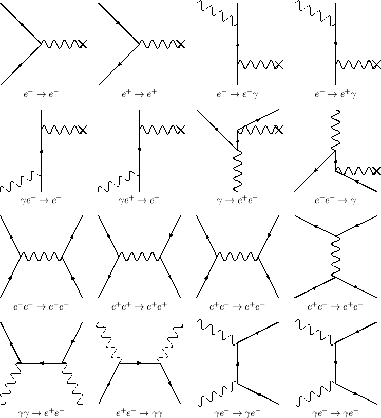
We will now develop the practical abilities to calculate lowest-order quantum electrodynamical processes (figure 7.1). That is, we will apply the propagator formalism to problems involving electrons, positrons, and photons. As we go, we will derive general rules for the calculation of transistion probabilities and cross sections: the Feynman rules.

Figure 7.1: Lowest order process involving a Coulomb field or two fermions.