


| Creating Multivariate Regression Trees (MRT) Using R-package |
riate Regression Trees is a technique originally described by De'ath (2002). This is a record of my personal journey in learning how to apply this technique to my data. I am sure there are better ways, and I hope by sharing my experiences others will share theirs to make this technique more useful. If you have any questions or suggestion feel free to contact me by email: Josh.Jacobs[at]ualberta.ca
Overview
I) Installing R-package and mvpart package from CRAN
II) Preparing Data and importing into R
III) Creating a MRT in R
IV) Hints and tricks
V) Notes and Problems
VI) References
I) Installing R-package and mvpart package from CRAN
1) Download and install the setup file from the r-project website
(at the time of writing the the setup file was available here)
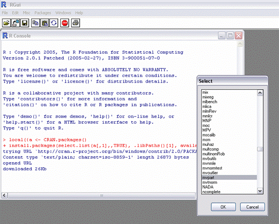
2) Open R and install the mvpart package by selecting Install package(s) from CRAN..
3) Select mvpart from the list and click OK
Now you are ready to do a MRT, but first you need to get your data into R!!!!

II) Preparing Data and importing into R
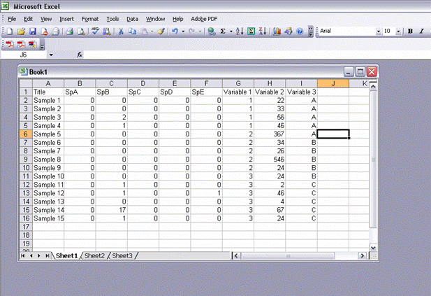
1) In Excel create a table with sites/samples/plots as row headings and species then independent variables as column headings.
2)Save the file as a .csv (comma separated values), by choosing "Save as" from the File menu, and change Save as type to "CSV(Comma delimited)"
You are now ready to import your data into R
3) Open the R program
4) Change the working directory to where you saved you .csv file from step 2 by selecting "Change dir" from the file menu and browsing to the proper directory
5) In order to import your file into R you need to use the read.csv command. To find out more about this command type "?read.csv" without the quotation marks at the pompt.To use the read.csv command type:
>name<- read.csv("filename.csv", row.names=1)
name: the name of the file in R
filename: the name you called your file in excel
row.names=1, use this if the first column of your data are the names of your rows (i.e."Sample 1")
III) Creating a MRT in R
1) Load the mvpart package by selecting "Load Package..." from the package menu. Then select "mvpart" and click ok.
2) Load you data by typing "Data (name)" at the command prompt (ie. "Data (MRT-Sample)"
3)To create a MRT using Euclidian distance measure, at the command line type:>mvpart(data.matrix(name[,1:12])~Variable 1+Variable 2+Variable 3+Variable 4+Variable 5+...,name)
(1:12 are the columns containing the species, Variable 1,2,3... are the names of the columns of the independent variables)
Try using the De'ath's (2002) data by using the commands;
>data (spider)
>mvpart(data.matrix(spider[,1:12])~herbs+reft+moss+sand+twigs+water,spider)View the mvpart help file by using the command;
>help (mvpart)4) To create a MRT using Bray-Curtis distance measure, at the command line type:
> mvpart(gdist(name[,1:12],meth="bray",full=TRUE,sq=TRUE)~Variable 1+Variable 2+Variable 3+Variable 4+Variable 5+...,name,method="mrt")
Try this using De'ath's (2002) data using the commands;
>data (spider)
>mvpart(gdist(spider[,1:12],meth="bray",full=TRUE,sq=TRUE)
~herbs+reft+moss+sand+twigs+water,spider,method="mrt",xv="pick",which="4")
IV) Hints and tricks
Interpretation of the Relative Error (RE) & Cross-Validated Error (CV-Error)
The Relative Error (RE) is described as the fit of the tree. Therefore, the variance explained by the tree is the inverse of the Error. However, the RE gives an over-optimistic view of how the tree will predict new data. This is better described by the CV-Error. The CV-error varies from 0 for a perfect predictor to 1 for a poor predictor (De'ath 2002).
Variance explained by each node
To find the variance explained by each node, write the results of the tree to a file a then find the summary of the file.
1) To write the results of the tree to a file, preceed the command line with name<- , just like went initially reading the csv.> mrtspider<- mvpart(gdist(spider[,1:12],meth="bray",full=TRUE,sq=TRUE)
~herbs+reft+moss+sand+twigs+water,spider,method="mrt",xv="1se", which="4")
2) Then find the summary of this file:
> summary(mrtspider)
3) The variance explained can be calculated from this table:
| CP | nsplit | rel error | xerror | xstd | |
| 1 | 0.556393 | 0 | 1 | 1.071913 | 0.125958 |
| 2 | 0.200243 | 1 | 0.443608 | 0.763165 | 0.154415 |
| 3 | 0.086731 | 2 | 0.243365 | 0.609107 | 0.175033 |
When "nsplit" is 0 the relative error is 1, so the variance explained (1-rel error) is 0.
When nsplit is 1 the relative error is 0.44, so the variance explained by the first split is 0.56
When nsplit is 2 the relative error is 0.24, so the variance explained by both splits is 0.76.
By simple subtraction the variance explained by just the second node is 0.20.
Identifying Indicator Species
The Indicator Species Analysis (ISA) (Dufrêne and Legendre 1997) is a helpful tool for characterizing the species at each node. To do this, I go back to the excel sheet and by sorting the data by the environmental variable for each split, I can assign each site to a node of the MRT. Then do a ISA using node as the grouping variable. I do this analysis in PCord still, but one day I will figure out how to do it in R and share it with the rest of the world.
Benefits of distance based MRTs (db-MRT)
Straight from De'ath (2002)
"...most forms of gradient analysis depend, either explicitly or implicitly, on a strong linear relationship between some measure of species dissimilarity and ecological distance. Analyses based on Euclidean distance often fail for moderate to long gradients, because compared to alternatives such as site standardized Bray-Curtis and extended dissimilarity, it is only weakly correlated with ecological distance."
V) Notes and Problems
- to make this method reliable I feel that a large number of trees should be run. For my personal application of this method I change the xv to equal "1se", so R will pick the best tree within one SE of the overall best, and get R to create a large number of trees (>50) and then pick the tree that is most consistently produced. There is probably a way to run make R run 100 trees and give a summary of the results.
- to make this method more useful you need to be able to create a table with the information seen in table 1 in De'ath's paper. I can not figure out how to reproduce this table and would really like too. I will keep trying to do this and will update this page when I can. If you know how to do this please let me know Josh.Jacobs[at]ualberta.ca
-the graphs produced in the MRT using Euclidian distance are the species across the x-axis and abundance across the y-axis. The graphs produced using Bray-Curtis Distance measure creates a different graph with species along the x-axis and I believe the sum of squares on the y-axis.
VI) References
De'Ath, G. 2002. Multivariate regression trees: a new technique for modeling species environment relationships. Ecology. 83:1105-1117.
Dufrêne, M., and P. Legendre. 1997. Species assemblages and indicator species: the need for a flexible asymmetrical approach. Ecological Monographs 67:345–366.
Last updated: 16 Jan 2007
Author: J Jacobs (Josh.Jacobs[at]ualberta.ca)