Orientation of parametric surfaces in \mathbb{R}^3

Section 5.5 Orientation of parametric surfaces in \(\mathbb{R}^3\)

Step 3, part II: we show that the parametrization of a surface induces an orientation on the image surface. However, this is a bit more subtle than for parametric curves, as not all surfaces are orientable. Thus we first discuss orientability of surfaces, and then show that the parametrization of an orientable surface induces an orientation on the image surface. We now focus on surfaces in \(\mathbb{R}^3\text{,}\) which are easier to visualize.

Objectives

You should be able to:

Define orientable and non-orientable surfaces.
Determine the orientation of a parametric surface in \(\mathbb{R}^3\text{.}\)
Relate the orientation of a parametric surface in \(\mathbb{R}^3\) to the normal vector.

Subsection 5.5.1 Orientable and non-orientable surfaces

In Section 5.2 we defined the orientation of \(\mathbb{R}^n\) and of a closed bounded region therein. We now want to define the orientation of a surface in \(\mathbb{R}^n\text{.}\) We will focus on a surface in \(\mathbb{R}^3\) in this section, since it is easier to visualize.

Recall from Definition 5.2.1 that the orientation of the vector space \(\mathbb{R}^n\) is given by a choice of “twirl”, specified by a choice of ordered basis on \(\mathbb{R}^n\text{.}\) For \(\mathbb{R}^2\text{,}\) this amounts to specifying a direction of rotation: either counterclockwise or clockwise. The canonical orientation is counterclockwise. The orientation of a closed, bounded, and simply connected region \(D \subset \mathbb{R}^n\) is the orientation induced by a choice of ordered basis on the ambient space \(\mathbb{R}^n\text{.}\)

Now suppose that \(\alpha:D \to \mathbb{R}^3\) is a parametric surface, with image surface \(S = \alpha(D) \subset \mathbb{R}^3\text{.}\) We would like to define an orientation on \(S\) in a way that is similar to what we did for the plane (or for \(D \subset \mathbb{R}^2\)) — we want to define a “direction of rotation” on the surface \(S\text{.}\) But this is not so obvious anymore, since \(S\) is a like a rubber sheet that can be bent, stretched, deformed, wrapped, what not. So what do we mean by direction of rotation?

The concept of tangent plane introduced in Definition 5.4.8 comes to the rescue. At each point \(p \in S\) (not on its boundary), the tangent plane \(T_p S\) is a two-dimensional vector space, i.e. \(\mathbb{R}^2\text{.}\) So we can naturally define a direction of rotation on the tangent plane at \(p \in S\) by specifying an ordered basis \(\{\mathbf{T}_u, \mathbf{T}_v \}\text{.}\) Then, we can define the orientation of the surface \(S\) by assigning an ordered basis to all tangent planes in a continuous manner.

When the surface is in \(\mathbb{R}^3\text{,}\) there is an equivalent way of defining a direction of rotation on the tangent planes. Instead of specifying an ordered basis for the tangent planes \(T_p S\text{,}\) we can specify a normal vector, as in Definition 5.4.9. If \(\mathbf{T}_u\) and \(\mathbf{T}_v\) form an ordered basis for the tanget plane \(T_p S\) at a point \(p \in S\text{,}\) then we define the normal vector

\begin{equation*} \mathbf{n} = \mathbf{T}_u \times \mathbf{T}_v. \end{equation*}

The ordering is important here, since this is what gives the direction of rotation. Changing from a direction of rotation to the opposite one amounts to exchanging the order of the two basis vectors, which, in turn, sends \(\mathbf{n}\) to \(- \mathbf{n}\text{.}\) So what matters here is the direction of the normal vector: it either points in one direction or the opposite direction, and this defines the two choices of orientation on the tangent plane at this point.

So we can think of an orientation of a surface as an assignment of a normal vector at all points on \(S\) in a continuous manner. Since what matters is the direction of the normal vector, choosing an assignment of a normal vector at all points on \(S\) is basically the same as choosing a side for the surface \(S\text{.}\) Which raises the following question: are all surfaces in \(\mathbb{R}^3\) orientable? That is, do all surfaces in \(\mathbb{R}^3\) have two sides?

Perhaps surprisingly, the answer is no! Not all surfaces are orientable. There exists surfaces that only have one side! We will come back to this in a second. Let us now define more carefully the notion of an “orientable surface”.

Definition 5.5.1. Orientable surfaces and orientation.

Let \(S \subset \mathbb{R}^3\) be a surface. We say that \(S\) is orientable if there exists a continuous function \(\mathbf{n}: S \to \mathbb{R}^3\) which assigns to all points \(p \in S\) (not on the boundary) the normal vector to the tangent plane \(T_p S\text{.}\) We say that it is non-orientable otherwise.

If \(S\) is orientable, then an orientation is a choice of continuous function \(\mathbf{n}: S \to \mathbb{R}^3\text{.}\) It assigns to all points on \(S\) a normal vector, which basically specifies one side of the surface (and also determines a direction of rotation on the tangent planes). Saying that the assignment of the normal vector is continuous amounts to saying that you pick the same side all around the surface — you do not suddenly jump from one side to the other.

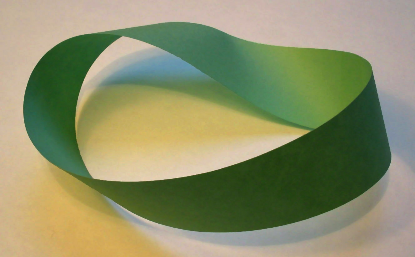
Most surfaces that we encounter in real life, such as spheres, cylinders, planes, tori, etc. are orientable. But the prototypical example of a non-orientable surface is the Möbius strip. This is a strange surface, shown in Figure 5.5.2. (It can be constructed by taking a long rectangle of paper, giving it one half-twist, and then taping back the ends together.) If you start at a point on the surface, you can pick a side, which amounts to defining a normal vector. Then you can move around the surface, always picking the same side. But at some point you will be back at the point you started with, but on the other side! (Try it!) So the assignment of normal vectors is not continuous, since you if you stopped just before the point you started with, the normal vector would suddenly have to jump from one side to the other.

What is going on? The point is that, on the Möbius strip, by doing this assignment of normal vectors, you end up labeling both sides of the strip. The reason is: the strip really only has one side! Crazy.

The Möbius strip is very cool, but from now on we will always assume that our surfaces are orientable.

Subsection 5.5.2 Orientation of a parametric surface

Now that we know how to define the orientation of a surface in \(\mathbb{R}^3\text{,}\) we can go back to our parametric surfaces. Are parametric surfaces naturally oriented? The answer is yes, as long as the image surface is assumed to be orientable (as we could, for instance, realize the Möbius strip as a parametric surface).

Lemma 5.5.3. Parametric surfaces are oriented.

Let

\begin{align*} \alpha: D \to\amp \mathbb{R}^3\\ (u,v) \mapsto\amp \alpha(u,v) = (x(u,v), y(u,v), z(u,v) ) \end{align*}

be a parametric surface, and assume that the image surface \(S = \alpha(D) \subset \mathbb{R}^3\) is orientable. The normal vector

\begin{equation*} \mathbf{n} = \mathbf{T}_u \times \mathbf{T}_v, \end{equation*}

with \(\mathbf{T}_u\) and \(\mathbf{T}_v\) the two tangent vectors from Definition 5.4.8, naturally induces an orientation on \(S\text{.}\)

Note that the order is important here: we must take the cross-product \(\mathbf{T}_u \times \mathbf{T}_v\) with the two vectors in the same order as the coordinates \((u,v)\) on \(D \subset \mathbb{R}^2\text{.}\)

Proof.

There isn't much to prove here. We showed in Definition 5.4.8 and Definition 5.4.9 that the normal vector was well defined (and non-zero) for all points that are not in the image of the boundary of \(D\text{.}\) So this gives a continuous assignment of a normal vector, and since we assume that \(S\) is orientable, it induces an orientation on \(S\text{.}\)

Remark 5.5.4.

As for parametric curves, there is another way of thinking about this statement. We can think of the parametrization \(\alpha: D \to \mathbb{R}^3\) as not only mapping the region \(D\text{,}\) but as also mapping its orientation. When we define parametric surfaces, we always think of the domain \(D\) as being given the canonical orientation (counterclockwise), which is induced by the canonical basis \(\{ \mathbf{e}_1, \mathbf{e}_2 \} \) on \(\mathbb{R}^2\text{,}\) with \(\mathbf{e}_1 = (1,0)\text{,}\) \(\mathbf{e}_2 = (0,1)\text{.}\) The vector \(\mathbf{e}_1\) points in the \(u\)-direction, and hence is mapped to \(\mathbf{T}_u\text{,}\) while the vector \(\mathbf{e}_2\) points in the \(v\)-direction and is mapped to \(\mathbf{T}_v\text{.}\) So the counterclockwise orientation on \(D\) induces the orientation given by the ordered basis \(\{ \mathbf{T}_u, \mathbf{T}_v \}\) on the tangent planes.

Finally, in Definition 5.2.9 we discussed the induced orientation on the boundary curve \(\partial D\) of a closed bounded region \(D\text{.}\) If \(D\) has canonical orientation, the induced orientation of the boundary is the direction of motion if you walk along the boundary curve keeping the region on your left. Similarly, a parametric surface induces an orientation on the boundary \(\partial S\) of the image surface \(S\text{.}\) Since for parametric surfaces we always start with the canonical orientation on \(D\text{,}\) we expect the induced orientation on the boundary of the image surface to be defined similarly, by walking along the boundary curve keeping the surface on your left. However, things are more subtle here, since the surface is in \(\mathbb{R}^3\text{,}\) so it's not immediately clear what it means to walk along the boundary keeping the surface your left... In which direction should your head be pointing?

For a region \(D \subset \mathbb{R}^2\text{,}\) we of course assumed that you were standing up. One way to think about this is that you had your head in the positive \(z\)-direction (if you assume that \(D\) is in the \(xy\)-plane embedded in \(\mathbb{R}^3\)). We now know that we can think of an orientation as a choice of normal vector, and the canonical orientation on the \(xy\)-plane corresponds to the normal vector pointing in the positive \(z\)-direction. In other words, we implicitly assumed that your head was pointing in the direction of the normal vector (or that you were walking on the side chosen by the orientation). This now generalizes to surfaces in \(\mathbb{R}^3\text{.}\)

Definition 5.5.5. Induced orientation on the boundary of a parametric surface.

Let \(\alpha: D \to \mathbb{R}^3\) be a parametric surface, with image surface \(S = \alpha(D)\) orientable and oriented by the parametrization. Let \(\partial S\) be the boundary (the edges) of the image surface \(S\text{.}\) The induced orientation on the boundary curve \(\partial S\) is the direction of travel if you keep the region on the left, with your head in the direction of the normal vector \(\mathbf{n} = \mathbf{T}_u \times \mathbf{T}_v\text{.}\) We denote by \(\partial \alpha\) the boundary of the image surface with its orientation induced by the parametrization \(\alpha\text{.}\)

Example 5.5.6. Upper half-sphere.

Let us realize the upper half-sphere of radius \(R\) as a parametric surface, and study its orientation and the induced orientation on its boundary.

The upper half-sphere has equation

\begin{equation*} x^2 + y^2 + z^2 = R^2, \end{equation*}

keeping only the points with \(z \geq 0\text{.}\) There are many ways that we can parametrize it. For instance, we can use either Cartesian or spherical coordinates. Let us do it in spherical coordinates, and leave the Cartesian coordinates parametrization for Exercise 5.5.4.1.

We recall from Example 5.4.5 the parametrization of the sphere of radius \(R\text{.}\) A parametrization of the upper half-sphere is obtained in the same way, but restricting the inclination angle \(\theta\) from \(0\) to \(\pi/2\text{.}\) We get the parametric surface \(\alpha: D \to \mathbb{R}^3\text{,}\) with

\begin{equation*} D = \{(\theta,\phi) \in \mathbb{R}^2~|~ \theta \in \left[ 0,\frac{\pi}{2} \right], \phi \in [0,2 \pi] \}, \end{equation*}

and

\begin{equation*} \alpha(\theta,\phi) = (R \sin(\theta) \cos(\phi), R \sin(\theta) \sin(\phi), R \cos(\theta) ). \end{equation*}

Now suppose that \(D\) has canonical orientation, as always for parametric surfaces. What is the induced orientation on the upper half-sphere? We calculate the tangent vectors:

\begin{align*} \mathbf{T}_\theta =\amp \left(R \cos(\theta) \cos(\phi), R \cos(\theta) \sin(\phi), - R \sin(\theta) \right)\\ \mathbf{T}_\phi =\amp \left(- R \sin(\theta) \sin(\phi), R \sin(\theta) \cos(\phi), 0 \right). \end{align*}

The normal vector is then:

\begin{equation*} \mathbf{n} = \mathbf{T}_\theta \times \mathbf{T}_\phi = R^2 \left( \sin^2(\theta) \cos(\phi), \sin^2(\theta) \sin(\phi), \sin(\theta)\cos(\theta) \right). \end{equation*}

The main question is the direction of the normal vector: does it point inwards (towards the center of the sphere), or outwards? In other words, is the orientation selecting the inner surface of the upper half-sphere or the outer surface? To find out, we only need to look at what happens at a given point on the upper half-sphere (we need to pick a point that is not in the image of the boundary of \(D\)). Let's pick the point with parameters \((\theta,\phi) = \left(\frac{\pi}{4}, 0 \right)\text{.}\) This is the point \(\frac{\sqrt{2}}{2} R \left( 1, 0, 1 \right)\text{.}\) At this point, the normal vector is:

\begin{equation*} \mathbf{n}\left(\frac{\pi}{4},0 \right) = \frac{R^2}{2} \left( 1,0,1 \right). \end{equation*}

We thus see that the normal vector points outwards in the radial direction, i.e. away from the origin. Therefore, the induced orientation on the upper half-sphere it outwards, i.e. the side of the surface selected is the outer surface.

What about the induced orientation on the boundary? The boundary of the upper half-sphere is the circle in the \(xy\)-plane with radius \(R\) (that's the edge of the upper half-sphere). In our parametrization, it corresponds to the points with parameters \((\theta,\phi) = \left(\frac{\pi}{2}, \phi \right)\) for \(\phi \in [0,2\pi]\text{.}\) The induced orientation should correspond to the direction of motion if we walk along the circle, with our head in the direction of the normal vector, keeping the surface on your left. As the normal vector point outwards, we are walking on the circle with our head pointing away from the origin. If we keep the surface on our left, we end up walking along the circle counterclockwise in the \(xy\)-plane. This is the induced orientation on the boundary circle.

Subsection 5.5.3 Orientation-preserving reparametrizations of a surface

Just as for parametric curves, there are many ways to parametrize a given surface \(S \subset \mathbb{R}^3\text{.}\) If we have a parametric surface \(\alpha: D \to \mathbb{R}^3\text{,}\) with

\begin{equation*} \alpha(u,v) = (x(u,v), y(u,v), z(u,v) ), \end{equation*}

and we think of \(u,v\) as functions of new variables \(s,t\text{,}\) then by doing this change of variable we may end up with a new parametrization of the same image surface. The question is whether this new parametrization induces the same orientation on the image surface or the opposite orientation.

Lemma 5.5.7. Orientation-preserving reparametrizations.

Let \(\alpha: D_1 \to \mathbb{R}^3\) be a parametric surface, with the image surface \(S = \alpha(C)\) orientable, and \(\alpha(u,v) = (x(u,v), y(u,v), z(u,v) )\text{.}\) Let \(D_2 \subset \mathbb{R}^2\) be another closed, bounded, and simply-connected region. Let \(\phi: D_2 \to D_1\) be a bijective and invertible function that can be extended to a \(C^1\)-function on an open subset \(U \subseteq \mathbb{R}^2\) that contains \(D_2\text{,}\) as in Definition 5.3.6. Then the pullback

\begin{align*} \phi^* \alpha: D_2 \amp \to \mathbb{R}^3\\ (s,t) \amp\mapsto (\phi^* x(s,t), \phi^* y(s,t), \phi^* z(s,t) ) = (x(\phi(s,t)), y(\phi(s,t)), z (\phi(s,t)) ) \end{align*}

is another parametrization of the same image surface \(S\text{.}\)

Furthermore, if \(\det J_\phi > 0\text{,}\) the induced orientation on \(S\) is the same for both parametrizations \(\alpha\) and \(\phi^* \alpha\text{,}\) and we say that the reparametrization is orientation-preserving. If \(\det J_\phi \lt 0\text{,}\) the two parametrizations \(\alpha\) and \(\phi^* \alpha\) have opposite orientations, and the reparametrization is orientation-reversing.

Proof.

First, it is clear that \(\alpha(D_1) = \phi^*\alpha(D_2)\text{,}\) i.e. the image surfaces are the same, since we are simply composing maps. But we need to show that \(\phi^* \alpha\) is a parametric surface, according to Definition 5.4.1.

Property 1 is clearly satisfied for \(\phi^*\alpha\) since \(\phi\) is assumed to be \(C^1\text{.}\) Property 3 is also satisfied, since \(\phi\) is bijective. As for Property 2, let us denote the tangent vectors to \(\phi^* \alpha\) by \(\mathbf{V}_s\) and \(\mathbf{V}_t\text{.}\) By definition,

\begin{align*} \mathbf{V}_s =\amp \frac{\partial}{\partial s}\phi^* \alpha(s,t) = \left( \frac{\partial x(\phi(s,t) )}{\partial s}, \frac{\partial y(\phi(s,t) )}{\partial s}, \frac{\partial z(\phi(s,t) )}{\partial s} \right),\\ \mathbf{V}_t =\amp \frac{\partial}{\partial t}\phi^* \alpha(s,t) = \left( \frac{\partial x(\phi(s,t) )}{\partial t}, \frac{\partial y(\phi(s,t) )}{\partial t}, \frac{\partial z(\phi(s,t) )}{\partial t} \right). \end{align*}

If we denote \(\phi(s,t) = (u(s,t), v(s,t))\text{,}\) using the chain rule, we get:

\begin{align*} \mathbf{V}_s =\amp \frac{\partial u}{\partial s} \left( \frac{\partial x(u,v)}{\partial u}, \frac{\partial y(u,v)}{\partial u}, \frac{\partial z(u,v)}{\partial u} \right) + \frac{\partial v}{\partial s} \left( \frac{\partial x(u,v)}{\partial v}, \frac{\partial y(u,v)}{\partial v}, \frac{\partial z(u,v)}{\partial v} \right)\\ =\amp \frac{\partial u}{\partial s} \mathbf{T}_u + \frac{\partial v}{\partial s} \mathbf{T}_v, \end{align*}

and, similarly,

\begin{align*} \mathbf{V}_t =\amp \frac{\partial u}{\partial t} \left( \frac{\partial x(u,v)}{\partial u}, \frac{\partial y(u,v)}{\partial u}, \frac{\partial z(u,v)}{\partial u} \right) + \frac{\partial v}{\partial t} \left( \frac{\partial x(u,v)}{\partial v}, \frac{\partial y(u,v)}{\partial v}, \frac{\partial z(u,v)}{\partial v} \right)\\ =\amp \frac{\partial u}{\partial t} \mathbf{T}_u + \frac{\partial v}{\partial t} \mathbf{T}_v. \end{align*}

Calculating the cross-product, we get:

\begin{align*} \mathbf{V}_s \times \mathbf{V}_t =\amp \left( \frac{\partial u}{\partial s} \frac{\partial v}{\partial t} - \frac{\partial v}{\partial s} \frac{\partial u}{\partial t} \right) \mathbf{T}_u \times \mathbf{T}_v\\ =\amp (\det J_\phi) \mathbf{T}_u \times \mathbf{T}_v. \end{align*}

Therefore, if \(\mathbf{T}_u\) and \(\mathbf{T}_v\) are linearly independent, then \(\mathbf{T}_u \times \mathbf{T}_v \neq 0\text{,}\) and since \(\phi\) is invertible, \(\det J_\phi \neq 0\text{.}\) Therefore \(\mathbf{V}_s \times \mathbf{V}_t \neq 0\text{,}\) and Property 2 is satisfied.

From this calculation we can also relate the induced orientations of the two parametrization \(\alpha\) and \(\phi^* \alpha\text{.}\) If we denote by \(\mathbf{n}\) the normal vector for \(\alpha\text{,}\) and \(\mathbf{m}\) the normal vector for \(\phi^* \alpha\text{,}\) from the calculation above we get:

\begin{equation*} \mathbf{m} = (\det J_\phi) \mathbf{n}. \end{equation*}

Thus, if \(\det J_\phi > 0\text{,}\) then the normal vectors of both parametrizations have the same sign (they pick the same side for the image surface) and the induced orientations are the same, while if \(\det J_\phi \lt 0\text{,}\) they have opposite signs (they pick opposite sides) and the induced orientations are opposite.

Exercises 5.5.4 Exercises

1.

Redo the parametrization of the upper half-sphere of radius \(R\text{,}\) as in Example 5.5.6, but in Cartesian coordinates. (The region \(D\) in this case should be a disk of radius \(R\text{.}\)) Find the induced orientation on the image surface by calculating the normal vector.

Solution.

The upper half-sphere of radius \(R\) is the surface in \(\mathbb{R}^3\) defined by the equation

\begin{equation*} x^2+y^2+z^2 = R^2 \end{equation*}

with \(z \geq 0\text{.}\) Since \(z \geq 0\text{,}\) we can solve explicitly for \(z\text{.}\) We get:

\begin{equation*} z = \sqrt{R^2 - x^2 - y^2}. \end{equation*}

This gives us another way of parametrizing the surface directly, since it is the graph of a function \(f(x,y) = \sqrt{R^2 - x^2- y^2}\text{.}\) We proceed as in Example 5.4.4. We find a parametrization \(\alpha: D \to \mathbb{R}^3\) with

\begin{equation*} \alpha(u,v) = (u,v,\sqrt{R^2 - u^2-v^2} ). \end{equation*}

However, we need to specify \(D\text{.}\) The region should be the disk that is at the bottom of the upper half-sphere, which is the disk of radius \(R\) centered at the origin. So the region \(D\) in the \((u,v)\)-plane should be given by \(u^2+v^2 \leq R^2\text{.}\) We can rewrite this as a \(u\)-supported region:

\begin{equation*} D = \{(u,v) \in \mathbb{R}^2\ | \ u \in [-R,R], - \sqrt{R^2 - u^2} \leq v \leq \sqrt{R^2-u^2}. \end{equation*}

To find the induced orientation, we need to calculate the normal vector. We first find the tangent vectors:

\begin{align*} \mathbf{T}_u =\amp \frac{\partial \alpha}{\partial u} = \left(1,0, - \frac{u}{\sqrt{R^2-u^2-v^2} } \right),\\ \mathbf{T}_v =\amp \frac{\partial \alpha}{\partial v} = \left(0,1, - \frac{v}{\sqrt{R^2-u^2-v^2} } \right). \end{align*}

The normal vector is given by the cross-product:

\begin{align*} \mathbf{n} =\amp \mathbf{T}_u \times \mathbf{T}_v\\ =\amp \left( \frac{u}{\sqrt{R^2-u^2-v^2} }, \frac{v}{\sqrt{R^2-u^2-v^2} }, 1 \right). \end{align*}

We need to determine in which direction it points (outwards of the sphere, or inwards), to determine the induced orientation. Let's pick the point on the sphere with parameters \((u,v) = (0,0)\text{.}\) This is the point \(\alpha(0,0) = (0,0,R)\text{,}\) which is the north pole. The normal vector at this point is \(\mathbf{n}(0,0) = (0,0,1)\text{.}\) It points upwards, that is, in the outwards direction (away from the origin, which is the center of the sphere). Therefore, this parametrization induces the orientation on the upper half-sphere given by a normal vector pointing outwards (it picks the outside of the surface).

We note that this is the same induced orientation as in Example 5.5.6. Indeed, we can relate the two parametrizations by the change of variables

\begin{equation*} (u,v) = (R \sin(\theta) \cos(\phi), R \sin(\theta) \sin(\phi) ). \end{equation*}

The determinant of the Jacobian of the transformation is

\begin{equation*} \det \begin{pmatrix} \frac{\partial u}{\partial \theta} \amp \frac{\partial u}{\partial \phi} \\ \frac{\partial v}{\partial \theta}\amp \frac{\partial v}{\partial \phi} \end{pmatrix} = \det \begin{pmatrix} R \cos(\theta) \cos(\phi) \amp - R \sin(\theta) \sin(\phi) \\ R \cos(\theta) \sin(\phi)\amp R \sin(\theta) \cos(\phi) \end{pmatrix} = R \sin(\theta) \cos(\theta), \end{equation*}

which is positive for \(\theta \in [0,\pi/2] \text{.}\) Therefore, the two parametrizations should induce the same orientation, as we found.

2.

Consider the surface \(S\) consisting of the part of the plane \(z + x + y = 2\) that lies inside the cylinder \(x^2 + y^2 = 1\text{.}\) Find two parametrizations of \(S\) that have opposite orientation.

Solution.

First, we can parametrize the plane by \(\alpha(u,v) = (u,v,2-u-v)\text{.}\) Now we need to find a region \(D\) in the \((u,v)\)-plane such that \(\alpha(D)\) is the part of the plane that lies inside the cylinder \(x^2+y^2=1\text{.}\) We see that if we take the region \(D\) to be the disk \(u^2+v^2=1\text{,}\) then the boundary circle of \(D\) is mapped to the boundary of the surface \(S\text{,}\) that is, the closed curve at the intersection of the plane and the cylinder. So this is the region \(D\) that we are looking for. We can realize it as a \(u\)-supported region. The final parametrization would be \(\alpha: D \to \mathbb{R}^3\) with

\begin{equation*} D = \{(u,v) \in \mathbb{R}^2\ | \ u \in [-1,1], - \sqrt{1-u^2} \leq v \leq \sqrt{1-u^2} \} \end{equation*}

and

\begin{equation*} \alpha(u,v) = (u,v,2-u-v). \end{equation*}

What is the induced orientation? The tangent vectors are:

\begin{equation*} \mathbf{T}_u = (1,0,-1), \qquad \mathbf{T}_v = (0,1,-1). \end{equation*}

The normal vector is

\begin{equation*} \mathbf{n} = \mathbf{T}_u \times \mathbf{T}_v = (1,1,1), \end{equation*}

which defines the induced orientation on the planar region \(S\text{.}\) (Note that it is a constant vector since the region \(S\) is planar (i.e. part of a plane), and so the normal direction is the same everywhere on \(S\text{.}\))

How can we find a second parametrization that has the opposite orientation? Well, there are many possibilities. But one easy way to get the normal vector to have opposite sign is to exchange the order of the two tangent vectors, i.e. exchange the variables \(u\) and \(v\text{.}\) In other words, we could define the parametrization \(\alpha_2: D \to \mathbb{R}^3\) with the same region \(D\) but

\begin{equation*} \alpha_2(u,v) = (v,u,2-u-v). \end{equation*}

(All we did is interchange \(u\) and \(v\) -- the image surface is obviously the same.) Then the tangent vectors are

\begin{equation*} \mathbf{T}_u = (0,1,-1), \qquad \mathbf{T}_v = (1,0,-1), \end{equation*}

and the normal vector is

\begin{equation*} \mathbf{n} = \mathbf{T}_u \times \mathbf{T}_v = (-1,-1,-1), \end{equation*}

which points in the opposite direction, and hence this parametrization induces the opposite orientation.

3.

We have seen in Example 5.4.4 how we can realize the graph of a function \(f(x,y)\) as a parametric surface in \(\mathbb{R}^3\text{.}\)

Show that the natural parametrization of Example 5.4.4 always induces an orientation on the graph of the function with normal vector pointing in the positive \(z\)-direction.
Find another parametrization of the graph of the function that induces the opposite orientation.

Solution.

(a) Let \(S \subset \mathbb{R}^3\) be the surface given by the graph \(z=f(x,y)\) of a function \(f\text{,}\) for some region \(D\) in the \((x,y)\)-plane. We parametrize it as \(\alpha: D \to \mathbb{R}^3\) with

\begin{equation*} \alpha(u,v) = (u, v, f(u,v) ), \end{equation*}

where \(D\) is the same region \(D\) but in the \((u,v)\)-plane. To calculate the normal vector, we calculate the tangent vectors:

\begin{equation*} \mathbf{T}_u = \left(1,0,\frac{\partial f}{\partial u} \right), \qquad \mathbf{T}_v = \left(0,1,\frac{\partial f}{\partial v} \right). \end{equation*}

The normal vector is given by the cross-product:

\begin{align*} \mathbf{n} =\amp \mathbf{T}_u \times \mathbf{T}_v\\ =\amp \det \begin{pmatrix} \mathbf{i} \amp \mathbf{j} \amp \mathbf{k} \\ 1 \amp 0 \amp \frac{\partial f}{\partial u} \\ 0 \amp 1 \amp \frac{\partial f}{\partial v} \end{pmatrix}\\ =\amp \left( -\frac{\partial f}{\partial u}, - \frac{\partial f}{\partial v} , 1 \right). \end{align*}

In particular, we see that it always points in the positive \(z\)-direction, regardless of the details of the function \(f\text{.}\)

(b) We can do just as in the previous question; we can exchange \(u\) and \(v\text{.}\) We can write a new parametrization as \(\alpha_2 :D_2 \to \mathbb{R}^3\text{,}\) with \(D_2\) being the same region as \(D\) but with \(u\) and \(v\) exchanged, and

\begin{equation*} \alpha(u,v) = (v, u, f(v,u) ). \end{equation*}

Then the tangent vectors are

\begin{equation*} \mathbf{T}_u = \left(0,1,\frac{\partial f(v,u)}{\partial u} \right), \qquad \mathbf{T}_v = \left(1,0,\frac{\partial f(v,u)}{\partial v} \right), \end{equation*}

and the normal vector is

\begin{equation*} \mathbf{n} = \mathbf{T}_u \times \mathbf{T}_v = \left( \frac{\partial f(v,u)}{\partial v} , \frac{\partial f(v,u)}{\partial u} , -1 \right), \end{equation*}

which is the same vector (with \(u\) and \(v\) exchanged) but with the opposite sign. This parametrization therefore induces the opposite orientation to the parametrization in (a).

4.

Consider the surface \(S\) consisting of the part of the cone \(z = \sqrt{x^2+y^2}\) between \(z = 1\) and \(z=5\text{,}\) with normal vector pointing outside the cone. The boundary \(\partial S\) of \(S\) consists in two separate oriented closed curves. Realize these two curves as parametric curves, with orientations that are consistent with the induced orientation on the boundary \(\partial S\text{.}\)

Solution.

The cone is shown in the figure below: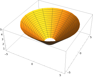

The surface. — Figure 5.5.8. The part of the cone \(z = \sqrt{x^2+y^2}\) between \(z=1\) and \(z=5\text{.}\)

The boundary has two components: the top boundary circle and the bottom boundary circle. If we call \(C_1\) the top boundary circle, and \(C_2\) the bottom one, then \(\partial S = C_1 \cup C_2\text{.}\) These two curves are given by the curves:

\begin{align*} C_1 =\amp \{(x,y,z) \in \mathbb{R}^3\ | \ x^2+y^2 = 25, z = 5 \},\\ C_2 =\amp \{(x,y,z) \in \mathbb{R}^3 \ | \ x^2+y^2 = 1, z=1 \}. \end{align*}

What is the induced orientation on these boundary curves? The surface of the cone is oriented with an outwards pointing normal vector. To get the induced orientation on the boundary curves, we should walk along the curves, keeping the region on our left, with our head pointing in the direction of the normal vector. We see that \(C_1\) should be oriented clockwise, while \(C_2\) should be oriented counterclockwise. We now want to find parametrization of these two curves that are consistent with the induced orientations.

We start with \(C_1\text{.}\) This is a circle of radius \(5\) in the plane \(z = 5\text{,}\) oriented clockwise. We can parametrize the circle using polar coordinates, but we want to use sine for \(x\) and cosine for \(y\) so that the resulting curve is oriented clockwise. We get the parametrization \(\alpha_1: [0,2 \pi] \to \mathbb{R}^3\) with

\begin{equation*} \alpha_1(\theta) = (5 \sin(\theta), 5 \cos(\theta), 5 ). \end{equation*}

As for \(C_2\text{,}\) it is the circle of radius \(1\) in the plane \(z=1\text{,}\) oriented counterclockwise. We use polar coordinates again, but cosine for \(x\) and sine for \(y\) so that it is oriented counterclockwise. We get \(\alpha_2: [0,2\pi] \to \mathbb{R}^3\) with:

\begin{equation*} \alpha_2(\theta) = (\cos(\theta), \sin(\theta), 1). \end{equation*}