Parametric surfaces in \mathbb{R}^n

Section 5.4 Parametric surfaces in \(\mathbb{R}^n\)

Step 3: we define parametric surfaces in \(\mathbb{R}^n\text{.}\) This is needed so that we can define integration of two-forms over surfaces in \(\mathbb{R}^n\) via pullback. The definition of parametric surfaces is similar to parametric curves, but there are new subtelties that appear, in particular in relation to the induced orientation on the surface.

Objectives

You should be able to:

Define parametric surfaces in \(\mathbb{R}^n\text{.}\)
Define the tangent plane to a parametric surface in \(\mathbb{R}^n\) at a point.
Use different parametrizations for the same surface.

Subsection 5.4.1 Parametric surfaces in \(\mathbb{R}^n\)

Definition 5.4.1. Parametric surfaces in \(\mathbb{R}^n\).

Let \(D \subset \mathbb{R}^2\) be a closed, bounded, and simply connected region. Let \(\partial D\) be its boundary, which is a simple closed curve. A parametric surface in \(\mathbb{R}^n\) is a vector-valued function:

\begin{align*} \alpha: D \to\amp \mathbb{R}^n\\ (u,v) \mapsto\amp \alpha(u,v) = (x_1(u,v), \ldots, x_n(u,v) ) \end{align*}

such that:

\(\alpha\) can be extended to a \(C^1\)-function on an open subset \(U \subseteq \mathbb{R}^2\) that contains \(D\text{;}\)
The tangent vectors
\begin{equation*} \mathbf{T}_u = \frac{\partial \alpha}{\partial u} = \left( \frac{\partial x_1}{\partial u}, \ldots, \frac{\partial x_n}{\partial u} \right), \qquad \mathbf{T}_v = \frac{\partial \alpha}{\partial v} = \left( \frac{\partial x_1}{\partial v}, \ldots, \frac{\partial x_n}{\partial v} \right) \end{equation*}
are linearly independent on the interior of \(D\text{.}\) (If \(n=3\text{,}\) this means that \(\mathbf{T}_u \times \mathbf{T}_v \neq 0\) on the interior of \(D\text{.}\))
If \(\alpha(u_1, v_1) = \alpha(u_2,v_2)\) for any two distinct \((u_1, v_1), (u_2, v_2) \in D\text{,}\) then \((u_1,v_1), (u_2,v_2) \in \partial D\text{.}\) In other words, \(\alpha\) is injective everywhere except possibly on the boundary of \(D\text{.}\)

The image \(S = \alpha(D)\) is a two-dimensional subspace of \(\mathbb{R}^n\text{,}\) which is the surface itself. We say that the parametric surface is smooth if \(\alpha\) can be extended to a smooth function on an open subset \(U \subseteq \mathbb{R}^2\) containing \(D\text{.}\)

This definition is obviously very similar to the definition of parametric curves in Definition 3.2.1. The three properties play similar roles: together, they ensure that the image surface \(S\) really looks like we expect a surface to look like, that is, some sort of sheet of rubber that may have been bent, deformed, warped, stretched, what not, but without introducing any puncture or tear. Property 3 ensures that our parametrization covers the image surface \(S\) exactly once (except possibly for boundary points). Property 2 also ensures that a parametrization induces a well defined choice of orientation on the image curve \(S\text{,}\) although this is more subtle than for parametric curves, as we will see in Section 5.5.

As for parametric curves, we can distinguish between two types of parametric surfaces, depending on whether the image surface is closed or not. It is a bit more subtle than for parametric curves, so let us look again at what it means for a parametric curve to be closed. In Definition 3.2.2, we said that a parametric curve \(\alpha:[a,b] \to \mathbb{R}^n\) is closed if the image curve \(C = \alpha([a,b])\) has no endpoints (it is a loop). If it is not closed, then we define the boundary \(\partial C = \{ \alpha(a), \alpha(b) \}\) as containing the endpoints of the image curve.

One way to think about a closed curve is that it is the boundary of a surface. In fact, one could say that a curve in \(\mathbb{R}^n\) is closed if and only if it forms the boundary of a surface. If it is not closed, then it must have endpoints, and those form the boundary of the image curve. This definition generalizes naturally to surfaces.

Definition 5.4.2. Closed parametric surfaces.

Let \(\alpha:D \to \mathbb{R}^n\) be a parametric surface with image surface \(S = \alpha(D) \subset \mathbb{R}^n\text{.}\) We say that the parametric surface is closed if and only if the image surface \(S\) is the boundary of a solid in \(\mathbb{R}^n\text{.}\) If it is not closed, then it must have edges: we call the set \(\partial S\) consisting of all the points on the edges of \(S\) the boundary of the surface.

Remark 5.4.3.

Given a parametric surface \(\alpha:D \to \mathbb{R}^n\text{,}\) one should not confuse \(\partial D\text{,}\) the boundary of the closed bounded region (the domain of \(\alpha\)), with \(\partial S\text{,}\) the boundary of the image surface. On the one hand, \(\partial D\) is never empty, as the domain of \(\alpha\) is a closed bounded domain -- in fact, \(\partial D\) is a simple closed curve in \(\mathbb{R}^2\) as we assume that \(D\) is simply connected. On the other hand, \(\partial S\) may or may not be empty, depending on whether the image surface is closed or not. Thus, generally, \(\alpha(\partial D) \neq \partial S\text{.}\) However, from the definition of parametric curves it follows that \(\partial S \subseteq \alpha(\partial D)\text{;}\) the points on the edges of \(S\) can only come from images of points on the boundary of the domain \(D\text{.}\)

Example 5.4.4. The graph of a function in \(\mathbb{R}^3\).

A large number of surfaces in \(\mathbb{R}^3\) can be obtained as the graph of a function \(f(x,y)\) of two variables:

\begin{equation*} z = f(x,y). \end{equation*}

This defines a surface in \(\mathbb{R}^3\text{.}\) If we choose \((x,y) \in D\) for some closed, bounded, simply connected domain \(D\text{,}\) then we can realize the surface as a parametric surface \(\alpha: D \to \mathbb{R}^3\) with

\begin{equation*} \alpha(u,v) = (u, v, f(u,v) ). \end{equation*}

Assuming that \(f: \mathbb{R}^2 \to \mathbb{R}\) is a \(C^1\) function, we can check that this satisfies the properties of a parametric surface. Property one is automatically satisfied, as \(f\) is \(C^1\text{.}\) The tangent vectors are

\begin{equation*} \mathbf{T}_u = \left(1,0, \frac{\partial f}{\partial u} \right), \qquad \mathbf{T}_v = \left(0,1,\frac{\partial f}{\partial v} \right). \end{equation*}

Those are clearly linearly independent, regardless of \(f\text{.}\) Finally, \(\alpha\) is certainly injective on the interior of \(D\text{;}\) in fact, it is injective everywhere on \(D\text{.}\)

Since \(\alpha\) is injective everywhere on \(D\text{,}\) including its boundary, this means that the image surface is not closed. In this case, its boundary \(\partial S = \alpha(\partial D)\) is the image of the boundary of the domain. Basically, the map \(\alpha\) takes the domain \(D\) and simply deform it continuously in the \(z\)-direction.

Surfaces realized as the graph of a function, as in the previous example, are very easy to study parametrically. But many surfaces do not arise in this way, and may instead be given by an implicit equation in \(\mathbb{R}^n\text{.}\) Finding a parametrization then becomes more difficult.

Example 5.4.5. The sphere.

As a second example, we consider the sphere of fixed radius \(R\) centered at the origin in \(\mathbb{R}^3\text{.}\) Its equation is

\begin{equation*} x^2 + y^2 + z^2 = R^2. \end{equation*}

We cannot think of this as the graph of a function as in the previous example, because we cannot solve for \(z\text{.}\) So we need to think a bit more to realize it as a parametric surface.

As this is a sphere, it is natural that spherical coordinates may be useful. A point on the sphere radius one can be written as

\begin{equation*} (x(\theta,\phi), y(\theta,\phi), z(\theta,\phi) ) = (R \sin(\theta) \cos(\phi), R \sin(\theta) \sin(\phi), R \cos(\theta) ). \end{equation*}

It is easy to see that

\begin{equation*} x(\theta,\phi)^2 + y(\theta,\phi)^2 + z(\theta,\phi)^2 = R^2, \end{equation*}

and thus those points lie on the sphere. Geometrically, \(\theta\) is the inclination angle from the \(z\) direction, and \(\phi\) is the azimuth angle measured counterclockwise from the \(x\)-axis. The inclination angle runs from \(0\) to \(\pi\text{,}\) while the azimuth angle runs from \(0\) to \(2 \pi\text{.}\)

Therefore, a realization of the sphere as a parametric surface is \(\alpha: D \to \mathbb{R}^3\text{,}\) with

\begin{equation*} D = \{(\theta,\phi) \in \mathbb{R}^2~|~ \theta \in [0,\pi], \phi \in [0,2 \pi] \}, \end{equation*}

and

\begin{equation*} \alpha(\theta,\phi) = (R \sin(\theta) \cos(\phi), R \sin(\theta) \sin(\phi), R \cos(\theta) ). \end{equation*}

We can check that it satisfies the properties of parametric surfaces. First, \(\alpha\) is smooth on \(\mathbb{R}^2\text{,}\) so Property 1 is fine. Second, it is easy to see geometrically that \(\alpha\) is injective everywhere, except at these points:

For any two \(\phi_1, \phi_2 \in [0,2 \pi]\text{,}\) \(\alpha(0,\phi_1) = \alpha(0,\phi_2) = (0,0,R)\text{.}\) All those points are mapped to the north pole of the sphere.
For any two \(\phi_1, \phi_2 \in [0,2 \pi]\text{,}\) \(\alpha(\pi,\phi_1) = \alpha(\pi,\phi_2) = (0,0,-R)\text{.}\) All those points are mapped to the south pole of the sphere.
For any \(\theta \in [0,\pi]\text{,}\) \(\alpha(\theta, 0) = \alpha(\theta, 2\pi) = (R \sin(\theta), 0, R \cos(\theta) )\text{.}\)

The important point is that these points where \(\alpha\) is not injective are all on the boundary of the rectangular region \(D\text{.}\) Therefore Property 3 is satisfied.

As for Property 2, the tangent vectors are

\begin{align*} \mathbf{T}_\theta =\amp (R \cos(\theta) \cos(\phi), R \cos(\theta) \sin(\phi), - R \sin(\theta) ),\\ \qquad \mathbf{T}_\phi =\amp (- R \sin(\theta) \sin(\phi), R \sin(\theta) \cos(\phi), 0). \end{align*}

Are those linearly independent? Since the \(z\)-coordinate of \(\mathbf{T}_\phi\) is zero, the only place where it could be a multiple of \(\mathbf{T}_\theta\) is when the \(z\)-coordinate of \(\mathbf{T}_\theta\) is also zero, that is \(- R \sin (\theta) = 0\text{.}\) This will only occur at \(\theta=0, \pi\text{,}\) which are on the boundary of \(D\text{.}\) So we conclude that the tangent vectors must be linearly independent on the interior of \(D\text{.}\) Alternatively, we could have calculated the cross-product \(\mathbf{T}_\theta \times \mathbf{T}_\phi\text{,}\) and showed that it does not vanish on the interior of \(D\text{.}\)

Finally, we note that the image surface, which is the sphere, is closed, since it is the boundary of a three-dimensional solid (the ball consisting of the interior of the sphere and its boundary).

Example 5.4.6. The cylinder.

Consider the lateral surface of a cylinder of fixed radius \(R\) extending in the \(z\)-direction. Suppose that we look at the part of the cylinder from \(z=0\) to \(z=2\) (we only look at the lateral surface of the cylinder, we do not include the top and the bottom). How do we realize it as a parametric surface?

The equation of the cylinder is

\begin{equation*} x^2 + y^2 = R^2, \end{equation*}

with \(z\) running from \(0\) to \(2\text{.}\) To parametrize it, we introduce polar coordinates. Then a point on the cylinder can be written as

\begin{equation*} S (x(\theta,w), y(\theta,w), z(\theta,w) ) = (R \cos(\theta), R \sin(\theta), w). \end{equation*}

If we restrict \(w\) from \(0\) to \(2\text{,}\) we get the parametric surface \(\alpha: D \to \mathbb{R}^3\) with

\begin{equation*} D = \{ (\theta,w) \in \mathbb{R}^2 ~|~ \theta \in [0,2 \pi], w \in [0,2] \}, \end{equation*}

and

\begin{equation*} \alpha(\theta,w) = (R \cos(\theta), R \sin(\theta), w). \end{equation*}

Does it satisfy the properties of a parametric surface? First, \(\alpha\) is smooth on \(\mathbb{R}^2\text{,}\) so Property 1 is satisfied. As for Property 2, \(\alpha\) is injective except at the points \(\alpha(0,w) = \alpha(2 \pi,w) = (R,0,w)\text{,}\) for all \(w \in [0,2]\text{.}\) But those are on the boundary of the rectangular region \(D\text{,}\) so it is fine. Finally, the tangent vectors are

\begin{equation*} \mathbf{T}_\theta = (- R \sin(\theta), R \cos(\theta), 0), \qquad \mathbf{T}_w = (0,0, 1). \end{equation*}

Those are clearly linearly independent everywhere, so Property 3 is satisfied.

The image surface here (the cylinder) is not closed; its boundary consists of its two edges, namely the circle at \(w=0\) and the circle at \(w=2\text{.}\)

Subsection 5.4.2 Grid curves

In order to help visualize a parametric surface \(\alpha: D \to \mathbb{R}^n\text{,}\) it is sometimes useful to sketch the grid curves on the image surface \(S = \alpha(D)\text{.}\) Suppose that \(D\) is a closed, simply connected, bounded domain in the \(uv\)-plane. The idea is to consider the horizontal and vertical lines in the \(uv\)-plane that lie on \(D\text{;}\) those are the lines \(u=u_0\) or \(v=v_0\) for constant \(u_0, v_0\text{.}\) The image of these lines under the map \(\alpha\) will be curves on the image surface \(S\text{:}\) those are called the grid curves. They help visualize how the parametrization \(\alpha\) maps the region \(D\) onto the image surface \(S\text{.}\)

Example 5.4.7. Grid curves on the sphere.

Consider the sphere of Example 5.4.5, which is realized as the parametric surface \(\alpha: D \to \mathbb{R}^3\) with

\begin{equation*} D = \{(\theta,\phi) \in \mathbb{R}^2~|~ \theta \in [0,\pi], \phi \in [0,2 \pi] \}, \end{equation*}

and

\begin{equation*} \alpha(\theta,\phi) = (R \sin(\theta) \cos(\phi), R \sin(\theta) \sin(\phi), R \cos(\theta) ). \end{equation*}

The domain \(D\) is a rectangular region. Horizontal lines on \(D\) correspond to lines with \(\phi = C\) for constants \(C\text{.}\) The image of the horizontal lines would be the grid curves

\begin{equation*} \alpha(\theta,C) = (R \cos(C) \sin(\theta), R \sin(C) \sin(\theta), R \cos(\theta) ). \end{equation*}

Since \(\theta\) is the inclination angle, those curves correspond to curves of constant longitude, starting at the north pole and ending at the south pole.

As for the vertical lines on \(D\text{,}\) they are given by the lines with \(\theta = K\) for constants \(K\text{.}\) The image of the vertical lines would be the grid curves

\begin{equation*} \alpha(K,\phi) = (R \sin(K) \cos(\phi), R \sin(K) \sin(\phi), R \cos(K) ). \end{equation*}

Those correspond to the curves of constant latitude, going all around the sphere.

Subsection 5.4.3 The tangent planes

Let \(\alpha: D \to \mathbb{R}^n\) be a parametric surface, and \(S = \alpha(D) \subset \mathbb{R}^n\) the image curve. In the definition of parametric surfaces Definition 5.4.1, we introduced the “tangent vectors”

\begin{equation*} \mathbf{T}_u = \frac{\partial \alpha}{\partial u} = \left( \frac{\partial x_1}{\partial u}, \ldots, \frac{\partial x_n}{\partial u} \right), \qquad \mathbf{T}_v = \frac{\partial \alpha}{\partial v} = \left( \frac{\partial x_1}{\partial v}, \ldots, \frac{\partial x_n}{\partial v} \right), \end{equation*}

but we did not really explain their geometric meaning.

At a point \(P \in S\text{,}\) there is a two-dimensional space of tangent directions to the surface. This is what is called the “tangent plane” to the surface at \(P \in S\text{.}\) It gives the best linear approximation of the surface at that point.

The claim is that the tangent plane at a point \(p \in S\) is the two-dimensional vector space spanned by the vectors \(\mathbf{T}_u\) and \(\mathbf{T}_v\text{.}\) Indeed, recall that the grid curves are the curves \(\alpha(u,C) \in S\) and \(\alpha(K,v) \in S\) for constant \(C,K\text{.}\) By definition of partial derivatives, it then follows that the vectors \(\mathbf{T}_u\) and \(\mathbf{T}_v\) are tangent vectors at the point \(p\) pointing in the direction of these grid curves. Furthermore, in the definition of parametric surfaces, we assume that \(\mathbf{T}_u\) and \(\mathbf{T}_v\) are linearly independent on the interior of \(D\text{.}\) Thus, for any point \(p \in S\) which is in the image of the interior of \(D\text{,}\) we know that the vectors \(\mathbf{T}_u\) and \(\mathbf{T}_v\) span a two-dimensional vector space. We can thus define the tangent planes for a parametric surface as follows:

Definition 5.4.8. Tangent planes to a parametric surface.

Let \(\alpha:D \to \mathbb{R}^n\) be a parametric surface, with image surface \(S = \alpha(D)\text{.}\) For any point \(p \in S\) which is in the image of the interior of \(D\text{,}\) we define the tangent plane \(T_p S\) at \(p\) to be the two-dimensional vector space spanned by the tangent vectors \(\mathbf{T}_u\) and \(\mathbf{T}_v\) at \(p\text{.}\) It provides the best linear approximation of the surface at that point.

If we now restrict to parametric surfaces in \(\mathbb{R}^3\text{,}\) then there is another way that we can specify the tangent plane at a point. We can always find the equation of a plane in \(\mathbb{R}^3\) by specifying a point on the plane and a normal (perpendicular) vector to the plane. Indeed, if \(\mathbf{n}\) is a vector normal to a plane, and \((x_0,y_0,z_0)\) is a point on the plane, then the equation of the plane is:

\begin{equation*} \mathbf{n} \cdot (x-x_0, y-y_0, z-z_0) = 0. \end{equation*}

Thus, given a parametric surface \(\alpha : D \to \mathbb{R}^3\) with image surface \(S = \alpha(D)\text{,}\) at a point \(p \in S\) we can specify the tangent plane by instead specifying the normal vector to the surface at that point. But what is the normal vector? Well, if \(\mathbf{T}_u\) and \(\mathbf{T}_v\) are both tangent vectors, then we know how to find a new vector that is perpendicular to both vectors: we take the cross-product! We get:

Definition 5.4.9. Normal vectors to a parametric surface in \(\mathbb{R}^3\).

\begin{equation*} \mathbf{n} = \mathbf{T}_u \times \mathbf{T}_v. \end{equation*}

We note here that this normal vector is not normalized, i.e. it does not have length one. To get a normalized vector we would divide by its norm. When we talk about the normalized normal vector later on, we will use the notation

\begin{equation*} \mathbf{\hat{n}} = \frac{\mathbf{T}_u \times \mathbf{T}_v}{|\mathbf{T}_u \times \mathbf{T}_v|}, \end{equation*}

to avoid ambiguity.

Exercises 5.4.4 Exercises

1.

Realize the part of the plane \(z = x-2\) that lies inside the cylinder \(x^2+y^2 = 4\) as a parametric surface.

Solution.

Let us first sketch a picture of what the surface should look like: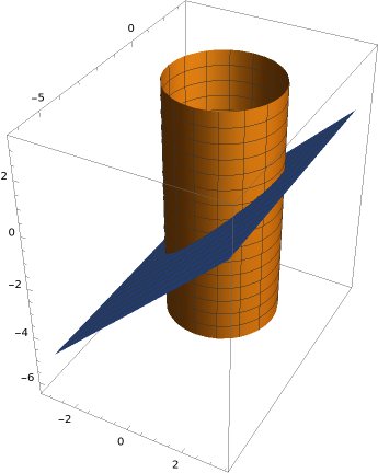

The surface \(S\) is the part of the blue plane that lies within the orange cylinder. How can we realize it as a parametric surface?

We first, we know how to parametrize the plane \(z = x- 2\text{.}\) The function

\begin{equation*} \alpha(u,v) = (u, v, u-2) \end{equation*}

is a parametrization of the plane. What we need to determine now is what is the region \(D\) in the \((u,v)\)-plane such that \(\alpha(D) = S\text{,}\) where \(S\) is the part of the plane contained within the cylinder \(x^2+y^2=4\text{.}\) What we can do is find the boundary curve of the surface \(S\text{,}\) which consists in the intersection of the plane \(z=x-2\) and the cylinder \(x^2+y^2=4\text{.}\) Using our parametrization above \(\alpha(u,v)\text{,}\) we see that \(x^2+y^2=4\) corresponds to the equation \(u^2+v^2=4\text{.}\) In other words, if we define \(D\) to be the disk of radius \(2\) centered at the origin, then \(\alpha\) maps its boundary (the circle of radius two) to the boundary of the surface \(S\text{,}\) and the interior to the interior. So this gives an appropriate choice of domain \(D\text{.}\) We can describe \(D\) as a \(u\)-supported region:

\begin{equation*} D = \{(u,v) \in \mathbb{R}^2\ | \ u \in [-2,2], - \sqrt{4-u^2} \leq v \leq \sqrt{4-u^2} \}. \end{equation*}

Then the surface \(S\) is realized as the parametric surface \(\alpha:D \to \mathbb{R}^3\text{,}\) with \(D\) above and \(\alpha(u,v) = (u,v,u-2)\text{.}\)

Note that there are many other parametrizations that we could have used. For instance, since the region \(D\) is a disk of radius \(2\text{,}\) we could have used polar coordinates. In other words, if we do the change of coordinates \(u = r \cos(\theta)\text{,}\) \(v = r \sin(\theta)\text{,}\) the region becomes

\begin{equation*} D_2 = \{(r,\theta) \in \mathbb{R}^2\ | \ r \in [0,2], \theta \in [0, 2\pi], \end{equation*}

and \(\alpha_2: D_2 \to \mathbb{R}^3\) with

\begin{equation*} \alpha_2(r, \theta) = (r \cos(\theta), r \sin(\theta), r \cos(\theta) - 2 ). \end{equation*}

That is another parametrization of the same surface \(S\text{.}\)

2.

Realize the part of the sphere \(x^2+y^2+z^2 = 4\) that lies above the cone \(z = \sqrt{x^2+y^2}\) as a parametric surface.

Solution.

Let us first sketch a picture of what the surface should look like: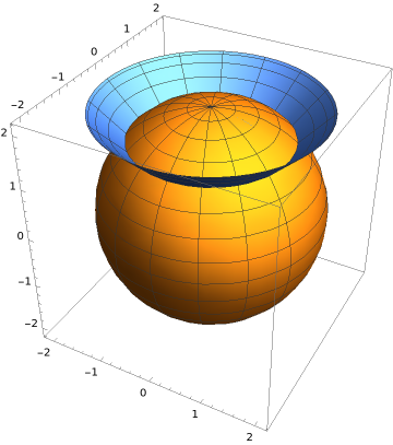

How can we realize \(S\) as a parametric surface?

We start by parametrizing the sphere of radius \(2\) centered at the origin. We use spherical coordinates. A parametrization for the sphere is \(\alpha: D \to \mathbb{R}^3\text{,}\) with

\begin{equation*} D = \{(\theta, \phi) \in \mathbb{R}^2\ | \ \theta \in [0,\pi], \phi \in [0,2\pi] \}, \end{equation*}

and

\begin{equation*} \alpha(\theta, \phi) = (2 \sin(\theta) \cos(\phi), 2 \sin(\theta) \sin(\phi), 2 \cos(\theta) ). \end{equation*}

This is a parametrization of the sphere, but this is not the surface we are interested in. We only want to keep the part of the sphere that lies above the cone \(z = \sqrt{x^2+y^2}\text{.}\) In other words, we want to restrict the range of the inclination angle \(\theta\) so that it only goes from \(0\) to the angle where the cone intersects the sphere. What is this angle? The cone has equation \(z = \sqrt{x^2+y^2}\text{.}\) Using our parametrization above for points on the sphere, we see that the points on the sphere that also lie on the cone (i.e. at the intersection of both surfaces) must satisfy

\begin{align*} 2 \cos(\theta) =\amp \sqrt{ (2 \sin(\theta) \cos(\phi) )^2 + (2 \sin(\theta) \sin(\phi))^2}\\ =\amp 2 \sin(\theta), \end{align*}

where we used the fact that \(\sin (\theta) \geq 0\) since \(\theta \in [0,\pi]\text{.}\) Therefore, we must have

\begin{equation*} \tan(\theta) = 1. \end{equation*}

The only solution with \(\theta \in [0,\pi]\) is \(\theta=\pi/4\text{.}\)

Therefore, we conclude that the region of the sphere that lies above the cone will be given by restricting the inclination angle to be between \(0\) and \(\pi/4\text{.}\) More precisely, a parametrization of our surface is given by \(\alpha_2: D_2 \to \mathbb{R}^3\text{,}\) with

\begin{equation*} D_2 = \{ (\theta,\phi) \in \mathbb{R}^2\ | \ \theta \in [0,\pi/4], \phi \in [0,2 \pi] \}, \end{equation*}

and

\begin{equation*} \alpha_2(\theta, \phi) = (2 \sin(\theta) \cos(\phi), 2 \sin(\theta) \sin(\phi), 2 \cos(\theta) ). \end{equation*}

3.

Consider the parametric surface \(\alpha: D \to \mathbb{R}^3\) with \(D = \{(u,v) \in \mathbb{R}^2\ | \ u \in [0,2], v \in [0,3] \} \) and

\begin{equation*} \alpha(u,v) = (u, v^3+1, u + v)\text{.} \end{equation*}

Find the tangent vectors \(\mathbf{T}_u\text{,}\) \(\mathbf{T}_v\text{,}\) and the normal vector \(\mathbf{n}\text{.}\)
Find an equation for the tangent plane to the image surface \(\alpha(D)\) at the point \((1,2,2)\text{.}\)

Solution.

(a) We calculate the tangent vectors by taking partial derivatives:

\begin{equation*} \mathbf{T}_u = \frac{\partial \alpha}{\partial u} = (1,0,1), \qquad \mathbf{T}_v = \frac{\partial \alpha}{\partial v} = (0, 3 v^2, 1). \end{equation*}

We find the normal vector by taking the cross-product of the tangent vectors:

\begin{align*} \mathbf{n} =\amp \mathbf{T}_u \times \mathbf{T}_v\\ =\amp \det \begin{pmatrix} \mathbf{i} \amp \mathbf{j} \amp \mathbf{k} \\ 1 \amp 0 \amp 1 \\ 0 \amp 3 v^2 \amp 1 \end{pmatrix}\\ =\amp (- 3 v^2, -1, 3 v^2). \end{align*}

(b) To find an equation of the tangent plane at the point \((1,2,2)\text{,}\) we use the point-normal form for the equation of a plane. First, we see that \(\alpha(1,1) = (1,2,2)\text{,}\) so the point is on the image surface \(\alpha(D)\) for the values of the parameters \((u,v) = (1,1)\text{.}\) The normal vector to the plane at that point is \(\mathbf{n}(1,1) = (-3,-1,3)\text{.}\) Then, by the point-normal form, we know that the equation of the tangent plane is

\begin{equation*} \mathbf{n} \cdot (x-1, y-2, z-2) = (-3,-1,3) \cdot (x-1, y-2, z-2) = 0. \end{equation*}

Evaluating the dot product, we get the equation of the tangent plane:

\begin{equation*} - 3 x - y + 3 z = 1. \end{equation*}

4.

Consider the curve \(y=x^2\) with \(x \in [0,2]\text{.}\) Find a parametrization for the surface obtained by rotating the curve about the \(y\)-axis.

Solution.

First, we sketch the curve \(y=x^2\) in the \((x,y)\)-plane inside \(\mathbb{R}^3\text{:}\)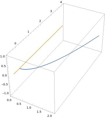

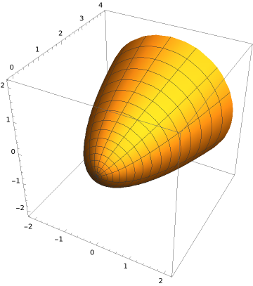
We rotate the curve about the \(y\)-axis, which is the orange line. After rotation, we get the following surface:

How do we parametrize this surface? Let's think about it. First, we can parametrize the curve \(y=x^2\) in the \((x,y)\)-plane within \(\mathbb{R}^3\text{,}\) with \(x \in [0,2]\text{,}\) by \(\phi(t) = (t, t^2,0)\) with \(t \in [0,2]\text{.}\) What happens if we rotate the curve about the \(y\)-axis? For a fixed value of \(t\text{,}\) the point with \((x,z)\)-coordinates \((t,0)\) gets rotated about the \(y\)-axis on a circle with radius \(t\text{.}\) We can thus parametrize this circle by \((x,z) = (t \cos(\theta), t \sin(\theta) )\text{,}\) with \(\theta \in [0, 2 \pi]\text{.}\) We do that for all values of \(t \in [0,2]\text{,}\) and we end up with the surface of revolution. The resulting parametrization is \(\alpha:D \to \mathbb{R}^3\) with

\begin{equation*} D = \{(t,\theta) \in \mathbb{R}^2\ |\ t \in [0,2], \theta \in [0, 2 \pi] \} \end{equation*}

and

\begin{equation*} \alpha(t,\theta) = (t \cos(\theta), t^2, t \sin(\theta) ). \end{equation*}