Section 5.2 Orientation of a region in \(\mathbb{R}^2\)
We proceed with building our theory of integration for two-forms. Step 1: we define the orientation of a closed bounded region in \(\mathbb{R}^2\text{,}\) the canonical orientation, and the induced orientation on its boundary.
Objectives
You should be able to:
Relate the orientation of \(\mathbb{R}^n\) to a choice of ordered basis.
Determine whether two choices of ordered bases on \(\mathbb{R}^n\) induce the same or opposite orientations.
Define the orientation of a closed bounded region in \(\mathbb{R}^2\text{.}\)
Determine the induced orientation on its boundary.
Subsection 5.2.1 Orientation of \(\mathbb{R}^n\)
Recall that a choice of orientation on \(\mathbb{R}\) is a choice of direction: either that of increasing real numbers, or of decreasing real numbers. We defined the direction of increasing real numbers as being the positive orientation, and called it the canonical orientation. We now generalize this to \(\mathbb{R}^n\text{.}\)
Definition 5.2.1. Orientation of \(\mathbb{R}^n\).
An orientation of the vector space \(\mathbb{R}^n\) is determined by a choice of ordered basis on \(\mathbb{R}^n\text{.}\) We think of the orientation as a “twirl”, which starts at the first basis vector, then rotates to the second basis vector, to the third, and so on and so forth. Ordered bases that generate the same twirl correspond to the same orientation of the vector space.
What this definition is saying is that to give an orientation to \(\mathbb{R}^n\text{,}\) we pick a choice of ordered basis. But not all ordered bases give rise to different orientations; if they generate the same twirl, they correspond to the same orientation of the vector space. If you think about it carefully (think about \(\mathbb{R}^2\) and \(\mathbb{R}^3\) first), you will see that for any \(\mathbb{R}^n\text{,}\) there are only two distinct choices of twirl, and hence only two distinct choices of orientation.
This is due to a basic fact in linear algebra. Any two ordered bases of \(\mathbb{R}^n\) are related by a linear transformation with non-vanishing determinant. One can see that two ordered bases that are related by a linear transformation with positive determinant generate the same twirl, while they generate opposite twirl if they are related by a linear transformation with negative determinant. So we can group oriented bases into two equivalence classes, depending on whether they are related by linear transformations with positive or negative determinants. These equivalence classes of oriented bases correspond to the two choices of orientation on \(\mathbb{R}^n\text{.}\)
Next we define the notion of canonical orientation.
Definition 5.2.2. Canonical orientation of \(\mathbb{R}^n\).
Let \((x_1, \ldots, x_n)\) be coordinates on \(\mathbb{R}^n\text{,}\) and \(\{ \mathbf{e}_1, \ldots, \mathbf{e}_n \}\) be the ordered basis
with \(\mathbf{e}_i\) the unit vector pointing in the positive \(x_i\)-direction. We call the orientation described by this ordered basis the canonical orientation of \(\mathbb{R}^n\) with coordinates \((x_1,\ldots,x_n)\text{,}\) and denote it by \((\mathbb{R}^n,+)\text{.}\) We denote by \((\mathbb{R}^n, -)\) the vector space \(\mathbb{R}^n\) with the opposite choice of orientation.
As always, the definition will be clearer with low-dimensional examples. First, let us show that we recover our previous definition of orientation in \(\mathbb{R}\text{.}\)
Example 5.2.3. Orientation of \(\mathbb{R}\) and choice of positive or negative direction.
If \(x\) is a coordinate on \(\mathbb{R}\text{,}\) the canonical orientation is specified by the basis vector \(\mathbf{e}_1 = 1\) in the positive \(x\)-direction. Thus the canonical orientation corresponds to the direction of increasing real numbers, as mentioned before. We denote it by \((\mathbb{R},+)\text{.}\)
Another choice of basis in \(\mathbb{R}\) would be \(\mathbf{f}_1=-1\text{.}\) It is related to \(\mathbf{e}_1\) by the linear transformation \(\mathbf{f}_1 = - \mathbf{e}_1\text{,}\) which has negative determinant. Thus \(\mathbf{f}_1\) generates the opposite orientation; indeed, it points in the direction of decreasing real numbers, which correspond to the orientation \((\mathbb{R},-)\text{.}\) So we recover our previous definition of orientation for \(\mathbb{R}\text{.}\)
Example 5.2.4. Orientation of \(\mathbb{R}^2\) and choice of counterclockwise or clockwise rotation.
Let \((x,y)\) be coordinates on \(\mathbb{R}^2\text{.}\) The canonical orientation is specified by the ordered basis \(\{ \mathbf{e}_1, \mathbf{e}_2 \}\text{,}\) with \(\mathbf{e}_1=(1,0)\) and \(\mathbf{e}_2=(0,1)\) being the unit vectors pointing in the positive \(x\)- and \(y\)-directions. In two dimensions, the twirl generated by an ordered basis corresponds to a choice of direction of rotation, from the first basis vector to the second. So one can think of an orientation of \(\mathbb{R}^2\) as being a choice of direction of rotation. We see that the canonical basis corresponds to the choice of counterclockwise rotation. Thus \((\mathbb{R}^2,+)\) corresponds to \(\mathbb{R}^2\) with the choice of counterclockwise rotation, which is the canonical orientation.
One could have instead chosen the ordered basis \(\{\mathbf{f}_1, \mathbf{f}_2 \} = \{ \mathbf{e}_2, \mathbf{e}_1 \}\) on \(\mathbb{R}^2\) (the order of the vectors is important). Rotating from \(\mathbf{e}_2\) to \(\mathbf{e}_1\) corresponds to a clockwise rotation, so this ordered basis should induce the opposite orientation \((\mathbb{R}^2,-)\text{.}\) Indeed, the two bases are related by the linear transformation (writing basis vectors as column vectors):
They therefore generate opposite orientations, as expected.
Example 5.2.5. Orientation of \(\mathbb{R}^3\) and choice of right-handed or left-handed twirl.
Let \((x,y,z)\) be coordinates on \(\mathbb{R}^3\text{.}\) The canonical orientation is specified by the ordered basis \(\{\mathbf{e}_1, \mathbf{e}_2, \mathbf{e}_3 \}\) with \(\mathbf{e}_1 = (1,0,0)\text{,}\) \(\mathbf{e}_2 = (0,1,0)\) and \(\mathbf{e}_3 = (0,0,1)\) being the unit vectors pointing in the positive \(x\)-, \(y\)- and \(z\)-directions. In three dimensions, the twirl generated by an ordered basis corresponds to a choice of left-handed or right-handed orientation. We can think of the first rotation from the first basis vector to the second as being represented by curling your fingers, and then the rotation from the second basis vector to the third as being in the direction of your thumb. The canonical basis thus corresponds to the choice of right-handed twirl, which is the canonical orientation on \(\mathbb{R}^3\) and denoted by \((\mathbb{R}^3,+)\text{.}\)
Another ordered basis on \(\mathbb{R}^3\) could have been \(\{ \mathbf{f}_1, \mathbf{f}_2, \mathbf{f}_3 \} = \{\mathbf{e}_2, \mathbf{e}_1, \mathbf{e}_3 \}\text{.}\) Following the twirl with your fingers and thumb, you will see that this corresponds to a left-handed twirl. So we expect it to correspond to the opposite orientation \((\mathbb{R}^3,-) \text{.}\) Indeed, it is related to the canonical basis by the linear transformation (writing basis vectors as column vectors):
The two ordered bases thus generate opposite orientations, as expected.
Subsection 5.2.2 Orientation of a closed bounded region in \(\mathbb{R}^2\)
Let us now focus on \(\mathbb{R}^2\text{.}\) Now that we defined the notion of orientation for the vector space \(\mathbb{R}^2\text{,}\) we can define the orientation of a closed bounded region in \(\mathbb{R}^2\text{,}\) just as we did for closed intervals in \(\mathbb{R}\text{.}\) But let us first define more carefully what we mean by a closed bounded region in \(\mathbb{R}^2\text{.}\) We use this to also recall the definition of path connectedness and simple connectedness (see Subsection 3.6.2), which will be useful later.
Definition 5.2.6. Regions in \(\mathbb{R}^2\).
Let \(D \subset \mathbb{R}^2\) be a region in \(\mathbb{R}^2\text{.}\)
A boundary point is a point \(p \in \mathbb{R}^2\) such that all disks centered at \(p\) contain points in \(D\) and also points not in \(D\text{.}\) We define the boundary of \(D\text{,}\) which we denote by \(\partial D\text{,}\) to be the set of all boundary points of the region \(D\text{.}\)
We say that a region \(D\) is closed if it contains all its boundary points, that is, \(\partial D \subseteq D\text{.}\) We say that it is open if it contains none of its boundary points, that is, \(D \cap \partial D = \emptyset\text{.}\)
We say that a region \(D\) is bounded if it is contained within a finite disk. In other words, it is bounded if it is finite in extent.
We say that a region \(D\) is path connected (or connected) if any two points in \(D\) can be connected by a path within \(D\text{.}\) In other words, it is path connected if it has only one component.
We say that a region \(D\) is simply connected if it is path connected and all simple closed curves (loops) in \(D\) can be continuously contracted to a point within \(D\text{.}\) In other words, it is simply connected if it has only one component and no holes.
Remark 5.2.7.
We will often consider closed, simply connected, bounded regions \(D \subset \mathbb{R}^2\text{.}\) Such a region can be constructed by considering a simple closed curve \(C \subset \mathbb{R}^2\text{,}\) and letting the region \(D\) be the closed curve and its interior. The boundary of the region is then \(\partial D = C\text{,}\) i.e. the closed curve that we started with. With this construction, it is clear that \(D\) is bounded, and it is simply connected since it has one component and no holes.
We note however that the closed curve \(C\) does not have to be a parametric curve; it may have kinks and corners, that is, it could be piecewise parametric. For instance, \(C\) could be a triangle, or a rectangle, etc. It needs to be simple however, i.e. not have self-intersection.
Next we define the orientation of a closed bounded region \(D \subset \mathbb{R}^2\text{.}\) Recall that we defined the orientation of a closed interval in \(\mathbb{R}\) as being a choice of direction, just as for \(\mathbb{R}\text{;}\) so we can think of the orientation of an interval as being induced by a choice of orientation on the surrounding vector space \(\mathbb{R}\text{.}\) We do the same for regions in \(\mathbb{R}^2\text{.}\)
Definition 5.2.8. Orientation of a closed bounded region in \(\mathbb{R}^2\).
Let \(D \subset \mathbb{R}^2\) be a closed bounded region in \(\mathbb{R}^2\text{,}\) and choose an orientation on \(\mathbb{R}^2\text{.}\) We define the orientation of the region \(D\) as being the orientation induced by the surrounding vector space \(\mathbb{R}^2\text{.}\) We write \(D_+\) for the region \(D \subset \mathbb{R}^2\) with the canonical (counterclockwise) orientation on \(\mathbb{R}^2\text{,}\) and \(D_-\) for the region with the opposite (clockwise) orientation. When we write \(D\) without specifying the orientation, we always mean the region \(D\) with its canonical orientation.
As a last step, given a closed bounded region \(D \subset \mathbb{R}^2\) with a choice of orientation, we need to define the induced orientation on its boundary \(\partial D\text{.}\) In the one-dimensional case, given a closed interval \([a,b] \in \mathbb{R}\) with canonical orientation, we defined the induced orientation on its boundary to be \(\{ (a,-), (b,+) \}\text{.}\) We do something similar in two dimensions. In this case, the boundary \(\partial D\) is a curve (which may have more than one components), and hence the induced orientation should be a choice of direction on each component.
Definition 5.2.9. Induced orientation on the boundary of a region in \(\mathbb{R}^2\).
Let \(D \subset \mathbb{R}^2\) be a closed bounded region with canonical orientation, and \(\partial D\) its boundary. Imagine that the region \(D\) is on the floor and that you are walking on its boundary. We define the induced orientation on each boundary component as being the direction of travel along the boundary keeping the region on your left. If \(D\) has the opposite orientation, the induced orientation on the boundary is the opposite direction of travel.
This will be clearer with some examples.
Example 5.2.10. Closed disk in \(\mathbb{R}^2\).
Consider the region
which is a disk of radius one centered at the origin. The boundary points in \(D\) are the points on the circle \(x^2+y^2=1\text{.}\) Thus \(\partial D\) is the circle of radius one centered at the origin. Since it is included in \(D\text{,}\) this means that \(D\) is closed. It is clearly bounded, as it can be contained within a disk. It is also simply connected.
We can give \(D\) the canonical orientation induced by the standard choice of ordered basis on \(\mathbb{R}^2\text{,}\) which is the choice of counterclockwise direction of rotation. The induced orientation on the boundary is the counterclockwise direction of motion along the circle, as this is the direction that one needs to move along the circle to keep its interior on the left.
Example 5.2.11. Closed square in \(\mathbb{R}^2\).
Consider the region
This corresponds to a square and its interior centered at the origin and with side length \(2\text{.}\) It is bounded as it can be contained within a finite disk. Its boundary \(\partial D\) is the square itself. As it is included in \(D\text{,}\) \(D\) is closed. It is also simply connected. If we choose the canonical orientation on \(D\text{,}\) the induced orientation on \(\partial D\) corresponds to moving counterclockwise along the square.
Example 5.2.12. Annulus in \(\mathbb{R}^2\).
Consider the region
This corresponds to an annulus with inner radius \(1\) and outer radius \(2\text{.}\) \(D\) is certainly bounded as it is contained within a finite disk. Its boundary has two components, \(\partial D = \partial D_1 \cup \partial D_2\text{,}\) where \(\partial D_1\) is the inner circle of radius \(1\) and \(\partial D_2\) is the outer circle of radius \(2\text{.}\) While the region is connected, it is not simply connected, as there is a hole in the middle.
Suppose that we choose the canonical orientation on \(D\text{.}\) What is the induced orientation on the boundary? We have to look at the two components separately. First, along the outer radius \(\partial D_2\text{,}\) we need to move in the counterclockwise direction to keep the interior of the annulus on the left. Thus the induced orientation is counterclockwise. However, for the inner circle \(\partial D_1\text{,}\) we need to move in the clockwise direction to keep the interior of the annulus on the left. So the induced orientation on \(\partial D_1\) is clockwise.
Remark 5.2.13.
There is another way that one can think of the induced orientation on the boundary of a region in \(\mathbb{R}^2\text{.}\) It is a little bit more subtle, and while it is not needed at this stage, it will be useful to generalize to regions in \(\mathbb{R}^3\) and \(\mathbb{R}^n\text{,}\) so let us mention it here.
Consider first the case where \(D \subset \mathbb{R}^2\) is a closed, simply connected, bounded region. Then \(\partial D\) is a simple closed curve. Since a curve is a one-dimensional subspace of \(\mathbb{R}^2\text{,}\) at a point \(p \in \partial D\) there are two choices of (length one) normal vectors: one that points “inwards” (towards \(D\)), and one that points “outwards” (away from \(D\)). For all points \(p \in \partial D\text{,}\) we pick the normal vector that points outwards. This defines an orientation on \(\partial D\) as follows; start with the normal vector, and rotate to a tangent vector in a way that reproduces the orientation (the twirl) on the ambient space \(\mathbb{R}^2\text{.}\) This defines a choice of tangent vector at all points on \(\partial D\text{,}\) which defines the induced direction of motion or orientation on the curve. It is easy to see in a figure that if the ambient space \(\mathbb{R}^2\) is equipped with canonical orientation, choosing the normal vectors pointing outwards corresponds to choosing the direction of motion keeping the region on the left.
If the region is not simply connected, its boundary may have many components. Do the same construction for each component, always choosing the normal vectors pointing outwards (away from \(D\)). This will induce the orientation on each component corresponding to the direction of motion keeping the region on the left.
This construction in terms of normal vectors is more subtle, but it directly generalizes to closed bounded regions in \(\mathbb{R}^n\text{,}\) which is nice.
Exercises 5.2.3 Exercises
1.
Determine whether the following regions are bounded, closed, connected, and/or simply-connected.
\(\displaystyle D = \{(x,y) \in \mathbb{R}^2~|~ x \geq 2, y \geq 3 \}.\)
\(\displaystyle D = \{(x,y) \in \mathbb{R}^2~|~ x^2 + y^2 \lt 1 \}.\)
\(\displaystyle D = \{(x,y)\in\mathbb{R}^2~|~ x \in [0,1] \cup [3,4], y \in [0,1] \}.\)
\(\displaystyle D = \{(x,y) \in \mathbb{R}^2~|~ \frac{x^2}{4} + \frac{y^2}{9} \leq 1 \}.\)
\(D\) extends forever in the positive \(x\) and \(y\) directions, so it is not bounded (it is not of finite extent). The boundary points are the points in \(D\) with \(x=2\) or \(y=3\text{,}\) since they are at the edge of the region. All those points are included in \(D\text{,}\) so \(D\) is closed. It is connected, as it has only one component, and it is simply-connected, as there is no hole.
\(D\) is the unit disk of radius one, without its boundary the circle of radius one. It is bounded, since it can be contained within a disk (it is of finite extent). It is not closed, since the boundary of \(D\) is the circle of radius one, which is not included in \(D\text{.}\) It is connected (one component) and simply-connected (no hole).
\(D\) consists in two separate square components. It is bounded, since the two square components can be contained within a disk (finite extent). It is closed, since the boundary points are the edges of the squares, which are all included in \(D\text{.}\) It is however not connected (two components), and hence also not simply-connected.
\(D\) is the region bounded by ellipse centered at the origin. It is bounded (finite extent), closed (the ellipse itself, which is the boundary, is included in \(D\)), connected (one component), and simply-connected (no hole).
2.
Let \(\{\mathbf{e}_1, \mathbf{e}_2, \mathbf{e}_3 \}\) be the canonical basis on \(\mathbb{R}^3\text{.}\) Show that the ordered basis \(\{\mathbf{e}_2, \mathbf{e}_3, \mathbf{e}_1 \}\) induces the same orientation on \(\mathbb{R}^3\) as the canonical basis.
To show that two ordered bases induce the same orientation, we need to show that they are related by a linear transformation with positive determinant. If we write \(\{ \mathbf{f}_1, \mathbf{f}_2, \mathbf{f}_3 \} = \{\mathbf{e}_2, \mathbf{e}_3, \mathbf{e}_1 \}\) for the ordered basis, we see that it is related to the canonical basis by the linear transformation (thinking of the basis vectors as column vectors):
Indeed,
But
and hence the two ordered bases induce the same orientation on \(\mathbb{R}^3\text{.}\)
3.
Let \(D\) be the upper half of a disk of radius one, including its boundary. Suppose that \(D\) is given the canonical orientation. Write its boundary, with the induced orientation, as an oriented parametric curve.
The upper half of a disk of radius one is the region of \(\mathbb{R}^2\) defined by:
Its boundary \(\partial D\) is the upper half of the circle, and the \(x\)-axis between \(x=-1\) and \(x=1\text{.}\) Since \(D\) has canonical orientation, the induced orientation corresponds to walking along the boundary curve keeping the region to the left, which means going counterclockwise along the boundary.
To realize \(\partial D\) as a parametric curve, we need to split it in two, since there are corners where the upper half disk meets the \(x\)-axis. Let \(C\) be the upper half disk, and \(L\) be the part of the \(x\)-axis in the boundary. We can parametrize the two curves separately. For \(C\) we take \(\alpha_1: [0,\pi] \to \mathbb{R}^2\) with
This has the correct orientation, as it goes counterclockwise around the circle. As for the \(L\text{,}\) we need to parametrize the line \(y=0\) from \(x=-1\) to \(x=1\text{.}\) We take \(\alpha_2: [-1,1] \to \mathbb{R}^2\) with
4.
Let \(A\) be a closed disk of radius four centered at the origin, and \(B\) be the region
Let \(D\) be the region that consists of all points in \(A\) that are not in \(B\text{.}\) Is \(D\) bounded? Closed? Connected? Simply-connected? What is the boundary of \(D\text{?}\) And if \(D\) is given the canonical orientation, what is the induced orientation on the boundary \(\partial D\text{?}\)
We note that \(B\) is the interior of a square of side length two centered at the origin. It is enclosed within \(A\text{,}\) which is a disk of radius four. Therefore, \(D\) is certainly bounded, since it is of finite extent.
The boundary points of \(D\) consists of all points on its outer boundary, which is the circle of radius four, and on its inner boundary, which consists on the points on the square centered at the origin. Thus, it has two separate components. But all the boundary points are included in \(D\text{,}\) and hence \(D\) is closed.
It is connected, as it has only one component. However, it is not simply connected, as any closed loop going around the inner missing square cannot be contracted to a point within \(D\text{.}\)
What is the induced orientation on the boundary? Let us denote by \(C_1\) the outer boundary consists of the circle of radius four, and \(C_2\) the inner boundary consisting of the square of side length two. Since \(D\) has canonical orientation, the induced orientation on the boundary will be obtained by walking along the boundary components keeping the region to the left. Along the outer boundary \(C_1\text{,}\) we will keep the region to the left if we walk counterclockwise. However, along the inner boundary \(C_2\text{,}\) we will keep the region to the left if we walk clockwise. Therefore, the induced orientation is councterclockwise on \(C_1\) and clockwise on \(C_2\text{.}\)
5.
The parametric curve \(\alpha: [0,\pi] \to \mathbb{R}^2\) with
is shown in the following figure:
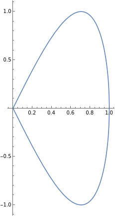
Suppose that \(D\) is the region consisting of the curve and its interior. What should the orientation of the region \(D\) be so that the induced orientation on its boundary is the same as the orientation of the parametric curve?
Let us first find the orientation of the parametric curve. The tangent vector is
In particular, at the origin, the tangent vector is \(\mathbf{T}(0) = (1, 2)\text{.}\) It points upwards and in the positive \(x\)-direction. Therefore, we see that the parametric curve has clockwise orientation.
The region \(D\) is the region consisting of the curve and its interior. If we walk clockwise along the curve, the region is on our right. This means that we must give \(D\) a clockwise (or negative) orientation if we want the induced orientation on the boundary to be the same as the orientation of the parametric curve.