Section 5.9 Applications of surface integrals
In this section we study some applications of surface integrals, such as calculating the flux of a vector field across a surface.
Objectives
You should be able to:
Determine and evaluate appropriate surface integrals and flux integrals in the context of applications in science.
Subsection 5.9.1 Surface integrals as flux integrals
The main interpretation of surface integrals consists in calculating the flux of a vector field across a surface in the direction of the normal vector. The easiest way to understand what this means is in terms of fluid mechanics.
Suppose that the vector field \(\mathbf{v}(x,y,z)\) is the velocity field of a fluid. Suppose that the function \(\rho(x,y,z)\) is the mass density of the fluid. Thus the vector field \(\rho \mathbf{v}\) is the rate of flow (mass per unit time) per unit area. We would like to calculate the rate of flow (mass per unit time) of fluid crossing a surface \(S\) in the normal direction \(\mathbf{n}\text{.}\) How can we do that?
We use the famous “divide and conquer”, or “slice it till you make it” process of integral calculus. We divide the surface \(S\) into tiny pieces of surface, and calculate the rate of flow through these tiny pieces of surface. Then we “sum over tiny pieces of surface”, and take the limit of an infinite number of pieces with infinitesimal size, which turns the calculation into a double integral.
More precisely, let \(dS\) be the area of a tiny piece of surface at \((x,y,z)\) on \(S\text{.}\) Assuming that \(S\) is a parametric surface, let
be the normalized normal vector at this point. Thus \(\rho \mathbf{v} \cdot \mathbf{\hat{n}}\) is the rate of flow per unit area in the normal direction at the point \((x,y,z)\text{.}\) Therefore, the rate of flow of fluid through this tiny piece of surface in the normal direction is
But... what is the area \(d S\text{?}\) We will come back to this in Section 7.2. Suppose that the tiny region of \(D\) that is mapped to the tiny piece of surface by the parametrization is a rectangle, with sides of lengths \(du\) and \(dv\text{.}\) We can think of these two sides as being vectors in the \(u\) and \(v\) directions with length \(du\) and \(dv\text{.}\) We can think of these vectors as being mapped by the parametrization to the rescaled tangent vectors \(du \mathbf{T}_u\) and \(dv \mathbf{T}_v\text{.}\) These two vectors span a parallelogram in the tangent plane, with area given by \(| du \mathbf{T}_u \times dv \mathbf{T}_v| = |\mathbf{T}_u \times \mathbf{T}_v| du dv\text{.}\) The idea is that the area of this parallelogram is a good approximation of the area \(dS\) of the tiny piece of surface, since the tangent plane is a good approximation of the surface. (And, when we sum over tiny pieces of surface and take the limit of the Riemann sum, this approximation will become exact.) As a result, we can write
for the area of the tiny piece of surface, with \(dA = du dv\text{.}\) Therefore, we get that the rate of flow of fluid through this tiny piece of surface in the normal direction is:
where \(\mathbf{n} = \mathbf{T}_u \times \mathbf{T}_v\) (not normalized).
The final step is to sum over tiny pieces of surfaces and take the limit of an infinite number of pieces of surface of infinitesimal area, which turns the sum into a double integral. The result is the double integral
which we recognize as the surface integral of the vector field \(\rho \mathbf{v}\text{!}\) Therefore, the surface of integral of \(\rho \mathbf{v}\) calculates the rate of flow of fluid across the surface in the normal direction.
While this was formulated for fluid velocity, one can study similar processes for other vector fields. The result is called the “flux” of the vector field.
Definition 5.9.1. The flux of a vector field across a surface.
Let \(\mathbf{F}(x,y,z)\) be a vector field on \(U \subseteq \mathbb{R}^3\text{,}\) and \(\alpha:D \to \mathbb{R}^3\) an oriented parametric surface with normal vector \(\mathbf{n}\text{.}\) The surface integral
is called the flux of \(\mathbf{F}\) across \(S\) in the normal direction \(\mathbf{n}\).
This is of course just the standard surface integrals that we have studied already. But it gives it an interpretation as calculating the flux of the vector field, which is why surface integrals are also known as “flux integrals”.
Subsection 5.9.2 Flux integrals beyond fluids
The main motivation for introducing the notion of flux is to calculate the rate of flow of a fluid across a surface. But the concept of flux is also important in other physical applications.
One such example is in electromagnetism. Suppose that \(\mathbf{E}(x,y,z)\) is an electric field. Then the surface integral
calculates what is known as the electric flux across the surface \(S\text{.}\) In fact, one of the important laws in electromagnetism is Gauss's law, which relates the electric charge to the flux of an electric field. More precisely, if \(S\) is a closed surface in an electric field \(\mathbf{E}\text{,}\) Gauss's law states that the net charge \(Q\) enclosed by the surface \(S\) is given by
i.e. it is the electric flux through \(S\) rescaled by a constant \(\epsilon_0\) known as the “permittivity of free space”. Here the surface \(S\) should be given the orientation of an outward normal vector.
Example 5.9.2. The electric flux and net charge of a point source.
Let \(q\) be a point charge at the origin. The electric force follows an inverse square law, that is, the magnitude of the electric field produced by the charge is inversely proportional to the square of the distance from the charge. More precisely, the electric field produced by the point charge is the vector field
Now suppose that you want to calculate the electric flux produced by the point charge across a sphere of radius \(R\) centered at the origin. By Gauss's law, this should calculate the total charge enclosed by the sphere. Since we only have a point charge at the origin, with charge \(q\text{,}\) we expect the electric flux to be given by \(q\text{.}\) Is that what we get?
The electric flux across the sphere in the outward direction is given by the flux integral
We already calculated such surface integrals in Exercise 5.6.4.5 using spherical coordinates. The result of this exercise applies here, with \(C = \frac{q}{4 \pi \epsilon_0}\text{.}\) We thus conclude that
In particular, Gauss's law states that the total charge enclosed by the sphere is
Phew!
We note that the flux does not depend on the radius of the sphere, as it should. In fact, we can go further. An argument very similar to Exercise 5.7.3.5 holds here as well, but using the divergence theorem (which we will explore in Section 6.2) instead of Green's theorem. The conclusion of the argument is that the flux of the electric field of a point charge at the origin across any closed surface that encloses the origin, not just the sphere, is always equal to \(q\text{,}\) as it should by Gauss's law. Cool!
The concept of flux is also used for instance in the study of heat flow. Suppose that the temperature at a point \((x,y,z)\) in a substance is given by the function \(T(x,y,z)\text{.}\) Then the heat flow is given the gradient of the temperature function, rescaled by a constant. More precisely, the heat flow is
where \(K\) is a constant called the conductivity of the substance. We are then often interested in calculating the rate of heat flow across a surface \(S\text{,}\) which is given by the flux of the vector field \(\mathbf{F}\) across \(S\text{:}\)
Exercises 5.9.3 Exercises
1.
Consider a fluid moving with velocity \(\mathbf{v}(x,y,z) = (-y, x, 0)\) and constant mass density \(\rho(x,y,z) = \rho_0\) with \(\rho_0\) a positive constant. (As we saw in Exercise 2.1.3.2, this type of fluid motion is a vortex in the \((x,y)\)-plane.) Show that the rate of flow of fluid across the cylinder \(x^2+y^2 = R^2\text{,}\) with \(-a \leq z \leq a\text{,}\) for some positive constants \(a,R\text{,}\) is zero. Explain why this result makes sense, looking at the fluid motion.
As we saw in Exercise 2.1.3.2, this type of fluid motion is a vortex in the \((x,y)\)-plane. Below is, first, a sketch of the velocity vector field of the fluid in 3 dimensions. But since there is no motion in the \(z\)-direction, I also present a two-dimensional plot of the vector field in the \((x,y)\)-plane, which makes the vortex motion more explicit.
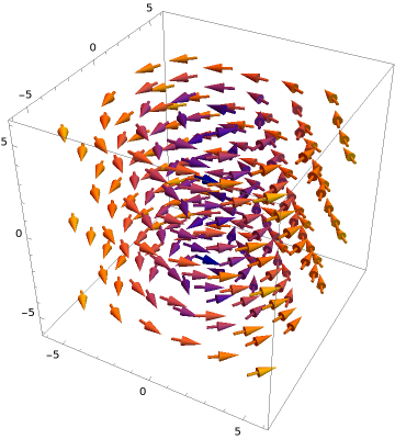
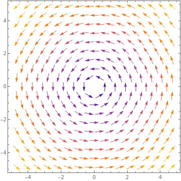
Looking at the two-dimensional figure, we see that the motion is moving around in a circular motion in the \((x,y)\)-plane about the origin. In three dimensions, since there is no motion in the \(z\)-direction, the fluid flow is circular about the \(z\)-axis. As such, if we imagine a cylinder centered on the \(z\)-axis in the fluid, we see that there is no fluid flowing across the surface of the cylinder. Thus we expect that the rate of flow of the fluid across the cylinder should be zero. Let us show this.
To calculate the rate of flow across the cylinder \(S\text{,}\) we need to evaluate the surface integral
We parametrize the surface of the cylinder as \(\alpha:D \to \mathbb{R}^3\) with
and
The tangent vectors are
The normal vector is
It is pointing inward, but it does not matter anyway which orientation we choose as we will show that the integral is zero. The surface integral is
This is just as we expected: there is no rate of flow of the fluid across the cylinder.
2.
Find the flux of the vector field
exiting the solid cone
To find the flux we need to evaluate the surface integral
where \(S\) is the surface boundary of the solid cone \(V\text{.}\)
The cone is shown in the figure below: 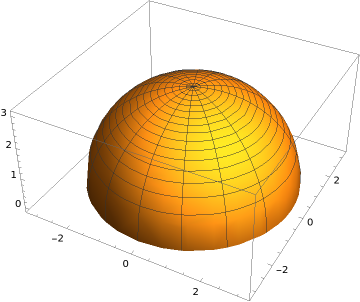
The boundary surface of \(V\) has two components: the lateral surface of the cone, which we will call \(S_1\text{,}\) and the bottom disk, which we will call \(S_2\text{.}\) We need to evaluate the surface integral on both components, and add up the results to calculate the flux of the vector field exiting the cone.
We parametrize \(S_1\) as \(\alpha_1: D_1 \to \mathbb{R}^3\) with
with
The tangent vectors are
The normal vector is
It points upward in the \(z\)-direction, and thus outward of the cone, as we want to calculate the flux exiting the cone. The surface integral is then
As for the bottom disk \(S_2\text{,}\) it is the disk \(x^2+y^2 \leq 9\) in the \(z=0\) plane. We can parametrize it as \(\alpha_2: D_2 \to \mathbb{R}^3\) with
and
The tangent vectors are
The normal vector is
which points downward, i.e. outward, which is what we want. The surface integral is
Thus there is no flux through the bottom of the cone.
We conclude that the flux exiting the cone is given by
3.
Use Gauss's law to find the net charge enclosed by the closed surface consisting of the cylinder \(x^2+y^2 = 1\text{,}\) \(-2 \leq z \leq 2\text{,}\) with its top and bottom, in the electric field \(\mathbf{E}(x,y,z) = (x, 0, 0).\)
To calculate the charge, by Gauss's law we need to calculate the eletric flux, that is, the surface integral of the electric field along the lateral surface of the cylinder as well as its top and bottom. To do so, we need to split the surface into three components. However, we can directly conclude that the surface integrals along the top and bottom of the cylinder will be zero. Why? The surface integrals calculate the flux of the vector field in the normal direction. That is, in the integrand we take the dot product of the vector field and the normal vector. For the top and bottom of the cylinder, we know that the normal vector will point in the \(z\)-direction (as the cylinder is centered around the \(z\)-axis). But the \(z\)-component of \(\mathbf{E}\) is zero, and therefore the integrand will vanish.
As a result, we only have to consider the lateral surface \(S\) of the cylinder, which we parametrize as \(\alpha:D \to \mathbb{R}^3\) with
and
The tangent vectors are
and the normal vector is
This is pointing inward, so we change the sign of the normal vector. The surface integral is then:
We conclude, by Gauss's law, that the net charge enclosed by the surface is
4.
Suppose that the temperature distribution in a substance in \(\mathbb{R}^3\) is given by the function
Show that the rate of heat flow along any horizontal plane \(z=C\text{,}\) where \(C\) is a constant, is zero. Explain why this is consistent with your expectation.
The heat flow is given by
To calculate the rate of heat flow across an horizontal plane \(z=C\text{,}\) we need to calculate the surface integral of the heat flow \(\mathbf{F}\) along the plane. In this process, we take the dot product of \(\mathbf{F}\) with the normal vector \(\mathbf{n}\) to extract the normal component of \(\mathbf{F}\text{.}\) Since the plane is horizontal, its normal vector will point in the \(z\)-direction. But the vector field \(\mathbf{F}\) has a vanishing \(z\)-component; therefore, \(\mathbf{F} \cdot \mathbf{n} = 0\text{,}\) and the surface integral along the horizontal plane will vanish.
This is consistent with our expectation because the temperature distribution does not depend on \(z\text{.}\) So it does not vary as we move in the \(z\)-direction; indeed, its gradient has a vanishing \(z\)-component. As a result, there is no heat flowing through horizontal planes, as we found.