One-forms and vector fields

Section 2.1 One-forms and vector fields

We define the concept of differential one-forms (or more simply one-forms), which will become the objects that can be integrated along curves in our theory of integration. We also define vector fields, and show that the two are closely connected: given a one-form, there is an associated vector field, and vice-versa.

Objectives

You should be able to:

Define one-forms and vector fields in $\mathbb{R}\text{,}$ $\mathbb{R}^2\text{,}$ and $\mathbb{R}^3\text{.}$
Translate between one-forms and vector fields.
Visualize a vector field in $\mathbb{R}^2$ by plotting vectors on a grid.

Subsection 2.1.1 One-forms

Let us start by defining one-forms in $\mathbb{R}\text{,}$ $\mathbb{R}^2\text{,}$ and $\mathbb{R}^3\text{.}$

Definition 2.1.1. One-forms.

A differential one-form (or simply one-form) on an open interval (or union of open intervals) $U \subseteq \mathbb{R}$ is an expression of the form

\begin{equation*} \omega = f(x)\ dx \end{equation*}

with $f: U \to \mathbb{R}$ a function with continuous derivatives (we say that the function $f$ is “smooth”, or $C^\infty\text{,}$ on $U$).

A one-form on an open subset¹ $U \subseteq \mathbb{R}^2$ is an expression of the form

\begin{equation*} \omega = f(x,y)\ dx + g(x,y)\ dy \end{equation*}

with $f,g: U \to \mathbb{R}$ functions with continuous partial derivatives (again, we say that they are smooth, or $C^{\infty}\text{,}$ on $U$).

A subset $U \subseteq \mathbb{R}^2$ is open if for every point $P \in U$ there is an open ball (an open disk in $\mathbb{R}^2\text{,}$ an open sphere in $\mathbb{R}^3$) centered at $P$ that lies entirely in $U\text{.}$ This is a generalization of open intervals (and unions of open integrals) to two and three dimensions.

A one-form on an open subset $U \subseteq \mathbb{R}^3$ is an expression of the form

\begin{equation*} \omega = f(x,y,z)\ dx + g(x,y,z)\ dy + h(x,y,z)\ dz \end{equation*}

for smooth functions $f,g,h: U \to \mathbb{R}\text{.}$

For the time being, you can think of the objects $dx\text{,}$ $dy$ and $dz$ as placeholders; they will be given an interpretation shortly. We remark here that the definition can easily be extended to $\mathbb{R}^n$ for any positive integer $n\text{,}$ but for the sake of simplicity, we will focus only on $n=1,2,3$ in this course.

We note here two obvious properties of one-forms, which follow from the definition.

If $\omega$ and $\eta$ are one-forms on $U\text{,}$ then the sum $\omega+\eta$ is also a one-form on $U\text{.}$
If $\omega$ is a one-form on $U$ and $f$ a smooth function on $U\text{,}$ then the product $f \omega$ is also a one-form on $U\text{.}$

Subsection 2.1.2 Vector fields

There is a closely related concept in vector calculus, which is called a vector field.

Definition 2.1.2. Vector fields.

A vector field on an open subset $U \subseteq \mathbb{R}^n$ is a function $\mathbf{F}: U \to \mathbb{R}^n\text{.}$ In other words, it is a rule which assigns to each point in $U \subseteq \mathbb{R}^n$ a vector with $n$ components.

For example, we can write a vector field $\mathbf{F}$ in $U \subseteq \mathbb{R}^2$ as

\begin{equation*} \mathbf{F}(x,y) = (f_1(x,y), f_2(x,y)), \end{equation*}

where $f_1, f_2$ are functions $f_1, f_2: U \to \mathbb{R}\text{.}$ We call these functions the component functions of the vector field. We say that the vector field is smooth if the component functions are smooth.

There are many examples of vector fields in physics: think of the velocity vector field of a moving fluid, or the gravitational force vector field produced by a mass.

Looking at the two definitions above, we see a natural correspondence between one-forms and vector fields.

Principle 2.1.3. Correspondence between one-forms and vector fields.

Given a one-form $\omega = f\ dx + g\ dy+ h\ dz\text{,}$ we can define an associated smooth vector field with component functions $(f,g,h)\text{.}$ Conversely, given a smooth vector field $\mathbf{F} = (f,g,h)\text{,}$ we can define an associated one-form $\omega = f\ dx + g\ dy + h\ dz\text{.}$

This is the starting point for the dictionary between the modern approach (one-forms) and the traditional approach (vector fields) to vector calculus.

Example 2.1.4. A one-form and its associated vector field.

The expression

\begin{equation*} \omega = x\ dx + x \sin(y) \ dy \end{equation*}

is a one-form on $\mathbb{R}^2\text{.}$ The associated vector field is the function $\mathbf{F}: \mathbb{R}^2 \to \mathbb{R}^2$ given by $\mathbf{F}(x,y) = (x, x \sin(y))\text{,}$ which assigns the vector $(x, x \sin(y)) $ to the point $(x,y) \in \mathbb{R}^2\text{.}$

Exercises 2.1.3 Exercises

1.

Consider the vector field in $\mathbb{R}^3$ given by $\mathbf{F}(x,y,z) = (x, \sin y, x y z)\text{.}$ Write the corresponding one-form.

Solution.

The corresponding one-form is $\omega = x \ dx + \sin y\ dy + x y z\ dz.$

2.

Consider the vector field $\mathbf{v}(x,y) = (-y, x) $ in $\mathbb{R}^2\text{.}$

Plot the given vector field at points with integer coordinates.
If the vector field represents the velocity of a flowing fluid, what kind of motion is this vector field describing?

Solution.

We can plot the vector field by plotting arrows for points in $\mathbb{R}^2$ with integer coordinates. For instance, at the point $(1,1)\text{,}$ the vector field would be the vector $\mathbf{v}(1,1) = (-1,1)\text{.}$ At $(0,1)\text{,}$ we would get $\mathbf{v}(0,1) = (-1,0)\text{.}$ And so on and so forth. The result is the following plot, which was obtained via this geogebra app.

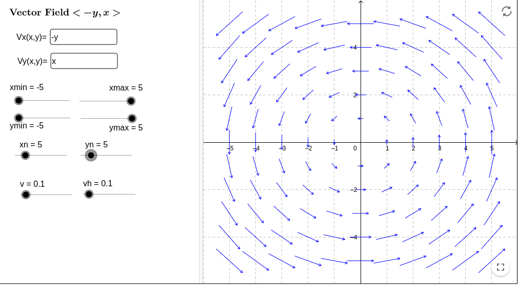
$A plot of the vector field $\mathbf{v}(x,y) = (-y, x)\text{.}$$

Figure 2.1.5. A plot of the vector field $\mathbf{v}(x,y) = (-y, x)\text{.}$
Looking at the plot, we see that the fluid is rotating around the origin counterclockwise. This type of fluid motion is called “vortex”.

3.

Consider a vector field $\mathbf{v}(x,y) = (5,1)\text{.}$ Suppose that it is the velocity field of a moving fluid. Suppose that you drop an object at the origin at time $t=0\text{.}$ Where will the object be at time $t=2\text{?}$

Solution.

The velocity field $\mathbf{v}(x,y) = (5,1)$ is constant, which means that all points in the fluid are moving at the same constant velocity. In other words, each point in the fluid is going through a linear motion of the form

\begin{equation*} \mathbf{x}(t) = \mathbf{x}_0 + t (5,1), \end{equation*}

where $\mathbf{x}_0$ is some initial position. If we drop an object at the origin at $t=0\text{,}$ its position vector is then described by $\mathbf{x}(t) = t (5,1)$ since its initial position is $\mathbf{x}_0 = (0,0)\text{.}$ We conclude that at time $t=2\text{,}$ the object is at position $\mathbf{x}(2) = 2(5,1) = (10,2)\text{.}$

4.

Consider the object $\omega = - \frac{y}{x^2+y^2}\ dx + \frac{x}{x^2+y^2}\ dy\text{.}$ Is this a one-form on $\mathbb{R}^2\text{?}$

Solution.

$\omega$ is not a one-form on $\mathbb{R}^2\text{,}$ because its component functions are not defined at the origin $(0,0) \in \mathbb{R}^2$ (we would be dividing by zero). However, it is a one-form on the open subset $U=\mathbb{R}^2 \setminus \{(0,0)\}$ where we removed the origin,² since the component functions are smooth on $U\text{.}$

The notation $\mathbb{R}^2 \setminus \{(0,0)\}$ means “$\mathbb{R}^2$ minus the point $(0,0)$”.