Green's theorem

Section 5.7 Green's theorem

Step 6: we study what happens if we integrate an exact two-form. We start by studying integrals of exact two-forms over bounded regions in

R^{2} :

this gives rise to Green's theorem.

🔗

Objectives

You should be able to:

State Green's theorem for integrals of exact two-forms over closed bounded regions in $R^{2} .$
Use Green's theorem to evaluate integrals of exact two-forms over closed bounded regions in $R^{2} .$
Use Green's theorem to evaluate line integrals of one-forms along simple closed curves in $R^{2} .$
Rephrase Green's theorem in terms of the associated vector fields.

🔗

Subsection 5.7.1 Green's theorem

🔗

Let us start by recalling the corresponding statement for integrals of exact one-forms over intervals in

R .

Let

f

be a zero-form on

U \subset R .

Let

[a, b] \in U

with the canonical orientation of increasing numbers. The boundary of the interval, with its induced orientation, is

\partial [a, b] = {(b, +), (a, -)} .

Then the integral of the exact one-form

ω = d f

along

[a, b]

can be evaluated as:

\int_{[a, b]} d f = \int_{\partial [a, b]} f = f (b) - f (a) .

🔗

This is nothing else but the Fundamental Theorem of Calculus, rewritten in a fancy way using one-forms and zero-forms.

🔗

We now want to do something similar for exact two-forms over closed bounded regions in

R^{2} .

🔗

Theorem 5.7.1. Green's theorem.

Let $η$ be a one-form on an open subset $U \subseteq R^{2} .$ Let $D \subset U$ be a closed bounded region with canonical orientation, and let $\partial D$ be its boundary with the induced orientation as in Definition 5.2.9. Then the integral of the exact two-form $d η$ along $D$ can be evaluated as:

\int_{D} d η = \int_{\partial D} η,

where on the right-hand-side this is understood as the integral of the one-form $η$ over the boundary curve $\partial D \subset R^{2},$ which is realized as a parametric curve (or union of parametric curves) compatible with the induced orientation.

We can be a little more explicit. If we write $η = f d x + g d y,$ then $d η = (\frac{\partial g}{\partial x} - \frac{\partial f}{\partial y}) d x \land d y .$ The statement of Green's theorem becomes

\int_{D} (\frac{\partial g}{\partial x} - \frac{\partial f}{\partial y}) d x \land d y = \int_{\partial D} (f d x + g d y) .

🔗

Proof.

We will only prove Green's theorem for recursively supported regions. (In fact, we will only write the proof for $x$ -supported regions, but the proof for $y$ -supported regions is analogous.) For more general closed bounded regions, one can prove Green's theorem by rewriting the region as an union of recursively supported regions.

We write $η = f d x + g d y$ and $d η = (\frac{\partial g}{\partial x} - \frac{\partial f}{\partial y}) d x \land d y .$

Let $D$ be an $x$ -supported region of the form:

D = {(x, y) \in R^{2} | x \in [a, b], u (x) \leq y \leq v (x)},

for some continuous functions $u, v : R \to R .$ The boundary $\partial D$ is a closed simple curve, with counterclockwise orientation. It can be split into four curves:

$C_{1}$ is the vertical line $x = b$ between $y = u (b)$ and $y = v (b);$
$C_{2}$ is the curve $y = v (x)$ between $x = b$ and $x = a;$
$C_{3}$ is the vertical line $x = a$ between $y = v (a)$ and $y = u (a);$
$C_{4}$ is the curve $y = u (x)$ between $x = a$ and $x = b .$

In fact, for $C_{2}$ and $C_{3},$ we will pick the opposite orientations (as it simplifies the parametrizations), and add a negative sign in front of the line integrals. Those four curves can be realized as parametric curves ( $C_{2}$ and $C_{3}$ have opposite orientations):

$α_{1} : [0, 1] \to R^{2}$ with $α_{1} (t) = (b, u (b) + (v (b) - u (b)) t);$
$α_{2} : [a, b] \to R^{2}$ with $α_{2} (t) = (t, v (t));$
$α_{3} : [0, 1] \to R^{2}$ with $α_{3} (t) = (a, u (a) + (v (a) - u (a)) t);$
$α_{4} : [a, b] \to R^{2}$ with $α_{4} (t) = (t, u (t));$

Calculating the pullbacks, we evaluate the line integrals:

\begin{aligned} \int_{α_{1}} η = & \int_{0}^{1} g (b, u (b) + (v (b) - u (b)) t) (v (b) - u (b)) d t, \\ \int_{α_{2}} η = & \int_{a}^{b} (f (t, v (t)) + g (t, v (t)) v^{'} (t)) d t, \\ \int_{α_{3}} η = & \int_{0}^{1} g (a, u (a) + (v (a) - u (a)) t) (v (a) - u (a)) d t, \\ \int_{α_{4}} η = & \int_{a}^{b} (f (t, u (t)) + g (t, u (t)) u^{'} (t)) d t . \end{aligned}

Putting those together, remembering that we need to add a negative sign for $C_{2}$ and $C_{3},$ we get:

\begin{aligned} \int_{\partial D} η = & \int_{α_{1}} η - \int_{α_{2}} η - \int_{α_{3}} η + \int_{α_{4}} η \\ = & \int_{0}^{1} (g (b, u (b) + (v (b) - u (b)) t) (v (b) - u (b)) - g (a, u (a) + (v (a) - u (a)) t) (v (a) - u (a))) d t \\ + \int_{a}^{b} (f (t, u (t)) - f (t, v (t)) + g (t, u (t)) u^{'} (t) - g (t, v (t)) v^{'} (t)) d t . \end{aligned}

Next, we need to evaluate the integral $\int_{D} d η .$ Here we will do our favourite trick: the pullback. Instead of using the $x$ -supported domain $D$ directly, we will pullback to a rectangular domain. This will allow us to integrate the two-form. Consider the function $ϕ : D_{2} \to D,$ where

D_{2} = {(s, t) \in R^{2} | s \in [a, b], t \in [0, 1]},

with

ϕ (s, t) = (s, u (s) + (v (s) - u (s)) t) .

We see that $ϕ (D_{2}) = D,$ and that the function is bijective. So by Lemma 5.3.7, we know that

\int_{D_{2}} ϕ^{*} (d η) = \int_{D_{1}} d η,

so we may as well calculate the left-hand-side. In fact, we also know that $ϕ^{*} (d η) = d (ϕ^{*} η) .$ So let us calculate this pullback. First,

ϕ^{*} η = f (ϕ (s, t)) d s + g (ϕ (s, t)) (u^{'} (s) + (v^{'} (s) - u^{'} (s)) t) d s + g (ϕ (s, t)) (v (s) - u (s)) d t .

Then

\begin{aligned} d (ϕ^{*} η) = & (- \frac{\partial f (ϕ (s, t))}{\partial t} - \frac{\partial}{\partial t} (g (ϕ (s, t)) (u^{'} (s) + (v^{'} (s) - u^{'} (s)) t)) \\ + \frac{\partial}{\partial s} (g (ϕ (s, t)) (v (s) - u (s)))) d s \land d t . \end{aligned}

Thus

\begin{aligned} \int_{D_{2}} ϕ^{*} (d η) = & \int_{a}^{b} \int_{0}^{1} (- \frac{\partial f (ϕ (s, t))}{\partial t} - \frac{\partial}{\partial t} (g (ϕ (s, t)) (u^{'} (s) + (v^{'} (s) - u^{'} (s)) t))) d t d s \\ + \int_{0}^{1} \int_{a}^{b} (\frac{\partial}{\partial s} (g (ϕ (s, t)) (v (s) - u (s)))) d s d t, \end{aligned}

where we used Fubini's theorem to exchange the order of two integrals in the second line. We can then evaluate the inner integrals using the Fundamental Theorem of Calculus, since they are definite integrals of derivatives. We get:

\begin{aligned} \int_{D_{2}} ϕ^{*} (d η) = & \int_{a}^{b} (f (ϕ (s, 0)) - f (ϕ (s, 1)) + g (ϕ (s, 0)) u^{'} (s) - g (ϕ (s, 1)) v^{'} (s)) d s \\ + \int_{0}^{1} (g (ϕ (b, t)) (v (b) - u (b)) - g (ϕ (a, t)) (v (a) - u (a))) d t . \end{aligned}

Substituting back the expression for $ϕ (s, t),$ we get:

\begin{aligned} \int_{D_{2}} ϕ^{*} (d η) = & \int_{a}^{b} (f (s, u (s)) - f (s, v (s)) + g (s, u (s)) u^{'} (s) - g (s, v (s)) v^{'} (s)) d s \\ + \int_{0}^{1} (g (b, u (b) + (v (b) - u (b)) t) (v (b) - u (b)) - g (a, u (a) + (v (a) - u (a)) t) (v (a) - u (a))) d t . \end{aligned}

Magic: this is exactly the same as the expression that we found many lines above for the line integral $\int_{\partial D} η!$ Woot woot! Therefore

\int_{D} d η = \int_{\partial D} η .

🔗

Remark 5.7.2.

If $D$ is simply connected, then $\partial D$ is a simple closed curve, and $D$ is the closed curve with its interior. In this case the line integral $\int_{\partial D} η$ is simply the line integral of the one-form $η$ along the simple closed curve with counterclockwise orientation.

However, in the statement of Green's theorem, $D$ can be more general. For instance, it could be an annulus. Then $\partial D$ would have two components: the inner and outer circle. The line integral $\int_{\partial D} η$ would then be the sum of the line integrals of the one-form $η$ along the two circles; the outer circle with counterclockwise orientation, and the inner circle with clockwise orientation, as this is the induced orientation on the boundary according to Definition 5.2.9.

🔗

Remark 5.7.3.

Following up on the previous remark, we note that we can read Green's theorem in two different ways, which is generally the case for all integral theorems of vector calculus. We could say:

The integral of the exact two-form $d η$ over the region $D \subset R^{2}$ with canonical orientation is equal to the integral of the one-form $η$ over the boundary $\partial D$ with the induced orientation.
The integral of the one-form $η$ over the simple closed curve $\partial D \subset R^{2}$ with canonical orientation is equal to the integral of its exterior derivative $d η$ over the interior $D$ with canonical orientation.

This is just two different readings of the same statement, depending on whether you start on the left-hand-side or the right-hand-side. Consequently, we can use Green's theorem either to evaluate integrals of exact two-forms via reading 1, or to evaluate line integrals over simple closed curves via reading 2.

In practice however, Green's theorem is generally useful mostly to evaluate line integrals by transforming them into surface integrals.

🔗

Example 5.7.4. Using Green's theorem to calculate line integrals.

Find the line integral of the one-form $ω = x y d x + (x + y) d y$ over the rectangle with vertices $(- 2, - 1), (2, - 1), (2, 0), (- 2, 0),$ with a clockwise orientation.

We could evaluate the line integral using previous techniques, by rewriting the curve as four parametric curves for each line segment and then use the definition of line integrals. But let us instead use Green's theorem.

Let us denote the rectangular curve by $C .$ It is the boundary of the region $D$ consisting of the interior of the rectangle with its boundary:

D = {(x, y) \in R^{2} | x \in [- 2, 2], y \in [- 1, 0]} .

Thus we can use Green's theorem to rewrite the line integral along $C$ as a surface integral over $D .$

We have to be careful with orientation though. If $D$ has canonical orientation, the induced orientation on the boundary rectangle $C$ will be counterclockwise. But the question is asking us to evaluate the line integral along $C$ with clockwise orientation. So in Green's theorem, if we relate the line integral to the surface integral over $D$ with canonical orientation, we will need to introduce a minus sign. More precisely, let us denote $C_{-}$ to be the rectangle with clockwise orientation, $C_{+}$ the rectangle with counterclockwise orientation, and $D$ the rectangular region with canonical (counterclockwise) orientation. Green's theorem states:

\int_{C_{-}} ω = - \int_{C_{+}} ω = - \int_{D} d ω .

So instead of calculating the line integral in the problem, we can calculate $- \int_{D} d ω .$

The two-form $d ω$ is:

d ω = x d y \land d x + d x \land d y = (1 - x) d x \land d y .

The integral can be evaluated:

\begin{aligned} \int_{D} d ω = & \int_{- 1}^{0} \int_{- 2}^{2} (1 - x) d x d y \\ = & \int_{- 1}^{0} {[x - \frac{x^{2}}{2}]}_{- 2}^{2} d y \\ = & \int_{- 1}^{0} (2 - (- 2) - 2 + 2) d y \\ = & 4 (0 - (- 1)) \\ = & 4. \end{aligned}

Therefore, the line integral of $ω$ along $C_{-}$ is

\int_{C_{-}} ω = - \int_{D} d ω = - 4.

It is a good exercise to check that this is the correct answer by evaluating the line integral using the standard approach with parametric curves.

🔗

While Green's theorem is mostly useful to evaluate line integrals, we can also use Green's theorem in the reverse direction, to evaluate integrals of exact two-forms. Here is an example.

🔗

Example 5.7.5. Area of an ellipse.

Find the area enclosed by the ellipse

\frac{x^{2}}{a^{2}} + \frac{y^{2}}{b^{2}} = 1.

The area is given by integrating the basic two-form $ω = d x \land d y$ over the region $D$ bounded by the ellipse with canonical orientation. We could calculate this integral directly, as a double integral. Or we can use Green's theorem, if $ω$ is exact. But it certainly is: for instance, we can write $ω = d η$ with $η = \frac{1}{2} (x d y - y d x)$ (we could choose other one-forms such that $d η = ω$ as well, but this one gives a nice and easy integral). Then Green's theorem states:

\int_{D} ω = \int_{C} η,

where on the right-hand-side we are evaluating the line integral of $η = \frac{1}{2} (x d y - y d x)$ along the ellipse with counterclockwise orientation.

We can parametrize the ellipse as $α : [0, 2 π] \to R^{2}$ with $α (t) = (a \cos (t), b \sin (t)) .$ The orientation is counterclockwise as required. The pullback $α^{*} η$ is:

α^{*} η = (\frac{a b}{2} \cos^{2} (t) - \frac{a b}{2} \sin (t) (- \sin (t))) d t = \frac{a b}{2} d t .

The line integral is then

\begin{aligned} \int_{C} η = & \int_{0}^{2 π} \frac{a b}{2} d t \\ = & π a b, \end{aligned}

which is the area of the ellipse.

🔗

Subsection 5.7.2 Vector form of Green's theorem

🔗

As always, we can translate our results to vector calculus concepts using our dictionary. It is a bit artificial though here, since Green's theorem really lives in two dimensions, while our vector calculus concepts live in three dimensions. But the idea is to think of the region

D

as being the trivial parametric surface in

R^{3}

where we embed it trivially in the

x y

-plane. That is,

α : D \to R^{3},

with

α (x, y) = (x, y, 0) .

The tangent vectors are

T_{x} = (1, 0, 0)

and

T_{y} = (0, 1, 0),

and the normal vector is of course

n = (0, 0, 1) = e_{3} .

🔗

To the one-form

η = f d x + g d y,

we associate the vector field

F = (f, g, 0) .

To the two-form

ω = d η

is then associated the vector field

\nabla \times F .

Using Corollary 5.6.5, we then see that we can rewrite the surface integral as

\int_{D} d η = \iint_{D} ((\nabla \times F) \cdot e_{3}) d A .

🔗

In other words, the integrand is the

z

-component of the curl

\nabla \times F .

🔗

As for the other side of Green's theorem, it is a line integral of the one-form

η

over the curve

\partial D .

Assuming that we parametrize the curve with a position function

r,

we can rewrite the line integral as

\int_{\partial D} η = \int_{\partial D} F \cdot d r .

🔗

The result is the vector form of Green's theorem:

\iint_{D} ((\nabla \times F) \cdot e_{3}) d A = \int_{\partial D} F \cdot d r .

🔗

Exercises 5.7.3 Exercises

🔗

1.

Evaluate the line integral of the one-form

ω = e^{y} d x + e^{x} d y

along the rectangle with vertices $(0, 0), (3, 0), (3, 2), (0, 2),$ counterclockwise, using two different methods: (a) directly, (b) using Green's theorem.

Solution.

(a) Let us call $\partial D$ the path along the rectangle counterclockwise. It is shown in the figure below.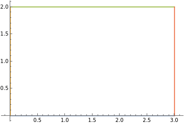

To evaluate the line integral directly, we need to parametrize separately the four line segments. We write the parametrizations as

α_{i} : [0, 1] \to R,

i = 1, \dots, 4,

with

\begin{aligned} α_{1} (t) = & (3 t, 0), \\ α_{2} (t) = & (3, 2 t), \\ α_{3} (t) = & (3 - 3 t, 2), \\ α_{4} (t) = & (0, 2 - 2 t) . \end{aligned}

We calculate the pullbacks:

\begin{aligned} α_{1}^{*} ω = & 3 d t, \\ α_{2}^{*} ω = & 2 e^{3} d t, \\ α_{3}^{*} ω = & - 3 e^{2} d t, \\ α_{4}^{*} ω = & - 2 d t . \end{aligned}

Putting all this together, the line integral becomes

\begin{aligned} \int_{\partial D} ω = & \int_{α_{1}} ω + \int_{α_{2}} ω + \int_{α_{3}} ω + \int_{α_{4}} ω \\ = & \int_{0}^{1} (3 + 2 e^{3} - 3 e^{2} - 2) d t \\ = & 1 + 2 e^{3} - 3 e^{2} . \end{aligned}

(b) We now use Green's theorem to calculate the line integral. By Green's theorem, we know that

\int_{\partial D} ω = \int_{D} d ω,

where $D$ is the interior of the rectangle with its boundary, that is,

D = {(x, y) \in R^{2} | x \in [0, 3], y \in [0, 2]},

with canonical orientation. We calculate the exterior derivative:

\begin{aligned} d ω = & e^{y} d y \land d x + e^{x} d x \land d y \\ = & (e^{x} - e^{y}) d x \land d y . \end{aligned}

The integral of the two-form is:

\begin{aligned} \int_{D} d ω = & \int_{D} (e^{x} - e^{y}) d x \land d y \\ = & \int_{0}^{2} \int_{0}^{3} (e^{x} - e^{y}) d x d y \\ = & \int_{0}^{2} (e^{3} - 1 - 3 e^{y}) d y \\ = & 2 e^{3} - 2 - 3 e^{2} + 3 \\ = & 1 + 2 e^{3} - 3 e^{2} . \end{aligned}

Therefore,

\int_{\partial D} ω = 1 + 2 e^{3} - 3 e^{2},

which is the same answer as in part (a), as it should.

🔗

2.

Use Green's theorem to evaluate the line integral of the vector field $F (x, y) = (x^{1 / 3} + y, x^{4 / 3} - y^{1 / 3})$ along the triangle with vertices $(1, 3), (2, 2), (1, 1),$ clockwise.

Solution.

Let us call $\partial D$ the path around the triangle clockwise. It is shown in the figure below.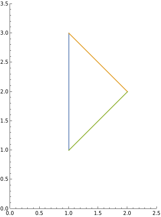

We associate to the vector field

F

the one-form

ω = (x^{1 / 3} + y) d x + (x^{4 / 3} - y^{1 / 3}) d y .

Since the path

\partial D

is oriented clockwise (negative orientation), by Green's theorem we know that

\int_{\partial D} ω = - \int_{D} d ω,

where $D$ is the interior of the triangle with its boundary, with canonical orientation. We can write equations for the three sides of the triangle. The blue line has equation $x = 1;$ the green line, $y = x;$ the orange line, $y = - x + 4 .$ Using these equations, we can describe $D$ as an $x$ -supported region:

D = {(x, y) \in R^{2} | x \in [1, 2], x \leq y \leq - x + 4} .

We calculate the exterior derivative $d ω :$

\begin{aligned} d ω = & d y \land d x + \frac{4}{3} x^{1 / 3} d x \land d y \\ = & (\frac{4}{3} x^{1 / 3} - 1) d x \land d y . \end{aligned}

Its integral along $D$ is:

\begin{aligned} \int_{D} d ω = & \int_{1}^{2} \int_{x}^{- x + 4} (\frac{4}{3} x^{1 / 3} - 1) d y d x \\ = & \int_{1}^{2} (\frac{4}{3} x^{1 / 3} - 1) [y]_{x}^{- x + 4} d x \\ = & \int_{1}^{2} (\frac{4}{3} x^{1 / 3} - 1) (- x + 4 - x) d x \\ = & \int_{1}^{2} (- \frac{8}{3} x^{4 / 3} + 2 x + \frac{16}{3} x^{1 / 3} - 4) d x \\ = & {(- \frac{8}{7} x^{7 / 3} + x^{2} + 4 x^{4 / 3} - 4 x)}_{x = 1}^{x = 2} \\ = & - \frac{32}{7} 2^{1 / 3} + 4 + 8 \cdot 2^{1 / 3} - 8 + \frac{8}{7} - 1 - 4 + 4 \\ = & \frac{3}{7} (8 \cdot 2^{1 / 3} - 9) . \end{aligned}

Therefore,

\int_{\partial D} ω = - \int_{D} d ω = - \frac{3}{7} (8 \cdot 2^{1 / 3} - 9) .

🔗

3.

Use Green's theorem to find the work done by the force

F (x, y) = (x^{2} + y^{2}, x y)

while moving an object first along the parabola $y = x^{2}$ from the origin to the point $(2, 4),$ then along a horizontal line back to the $y$ -axis, and then back to the origin along a vertical line.

Solution.

We denote the closed path by $\partial D .$ It is shown in the figure below.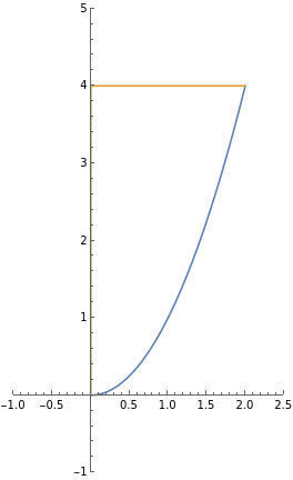

From the description of the path we know that the object is moving counterclockwise along the path. Therefore, if we associate the one-form

ω = (x^{2} + y^{2}) d x + x y d y

to the vector field

F,

by Green's theorem we know that

\int_{\partial D} ω = \int_{D} d ω,

with $D$ being the region enclosed by the path (with its boundary), with canonical orientation. The region $D$ can be described as an $x$ -supported region:

D = {(x, y) \in R^{2} | x \in [0, 2], x^{2} \leq y \leq 4} .

The exterior derivative $d ω$ is:

\begin{aligned} d ω = & 2 y d y \land d x + y d x \land d y \\ = & - y d x \land d y \end{aligned}

Its integral along $D$ is:

\begin{aligned} \int_{D} d ω = & - \int_{D} y d x \land d y \\ = & - \int_{0}^{2} \int_{x^{2}}^{4} y d y d x \\ = & - \int_{0}^{2} {[\frac{y^{2}}{2}]}_{y = x^{2}}^{y = 4} d x \\ = & - \int_{0}^{2} (8 - \frac{x^{4}}{2}) d x \\ = & - (16 - \frac{16}{5}) \\ = & - \frac{64}{5} . \end{aligned}

Therefore, by Green's theorem, the work done by the force $F$ while moving an object along the path $\partial D$ is:

\int_{\partial D} ω = - \frac{64}{5} .

🔗

4.

Suppose that a polygon has vertices $(x_{1}, y_{1}), (x_{2}, y_{2}), \dots, (x_{n}, y_{n}),$ in counterclockwise order. The area $A$ of the polygon is given by integrating the basic two-form $ω = d x \land d y$ over the polygon. Use Green's theorem to show that

A = \frac{1}{2} ((x_{1} y_{2} - x_{2} y_{1}) + (x_{2} y_{3} - x_{3} y_{2}) + \dots + (x_{n - 1} y_{n} - x_{n} y_{n - 1}) + (x_{n} y_{1} - x_{1} y_{n})) .

This is a well known formula for the area of an arbitrary polygon, see for instance https://en.wikipedia.org/wiki/Polygon#Area.

Solution.

We denote by $\partial D$ the closed path that goes around the polygon counterclockwise. It consists of $n$ line segments $L_{i},$ $i = 1, \dots, n,$ with $L_{i}$ being the line segment between the points $(x_{i}, y_{i})$ and $(x_{i + 1}, y_{i + 1})$ (for simplicity of notation, we define $(x_{n + 1}, y_{n + 1}) := (x_{1}, y_{1})$ ).

Further, we notice that the two $ω = d x \land d y$ is exact. We write it as $ω = d η$ for the one-form

η = x d y .

Note that this is certainly not the only choice of $η,$ but any $η$ such that $d η = ω$ will work.

Then, by Green's theorem, we know that the area $A$ of the polygon is given by

\begin{aligned} A = & \int_{D} d x \land d y \\ = & \int_{\partial D} η \\ = & \sum_{i = 1}^{n} \int_{α_{i}} η, \end{aligned}

where in the last line $α_{i}$ is a parametrization of the line segment $L_{i} .$ More explicitly, since the line segment $L_{i}$ joins the points $(x_{i}, y_{i})$ and $(x_{i + 1}, y_{i + 1}),$ we can parametrize it as $α_{i} : [0, 1] \to R^{2}$ with

α_{i} (t) = (x_{i} + t (x_{i + 1} - x_{i}), y_{i} + t (y_{i + 1} - y_{i})) .

Then

α_{i}^{*} η = (x_{i} + t (x_{i + 1} - x_{i})) (y_{i + 1} - y_{i}) d t .

The line integral along $α_{i}$ is then:

\begin{aligned} \int_{α_{i}} η = & \int_{0}^{1} (x_{i} + t (x_{i + 1} - x_{i})) (y_{i + 1} - y_{i}) d t \\ = & (y_{i + 1} - y_{i}) (x_{i} + \frac{1}{2} (x_{i + 1} - x_{i})) \\ = & \frac{1}{2} (y_{i + 1} - y_{i}) (x_{i} + x_{i + 1}) \\ = & \frac{1}{2} (x_{i} y_{i + 1} - x_{i + 1} y_{i} + x_{i + 1} y_{i + 1} - x_{i} y_{i}) . \end{aligned}

Finally, we add up these line integrals to get the area of the polygon. We get:

\begin{aligned} A = & \sum_{i = 1}^{n} \int_{α_{i}} η \\ = & \frac{1}{2} \sum_{i = 1}^{n} (x_{i} y_{i + 1} - x_{i + 1} y_{i} + x_{i + 1} y_{i + 1} - x_{i} y_{i}) \\ = & \frac{1}{2} ((x_{1} y_{2} - x_{2} y_{1} + x_{2} y_{2} - x_{1} y_{1}) + (x_{2} y_{3} - x_{3} y_{2} + x_{3} y_{3} - x_{2} y_{2}) + \dots \\ + (x_{n} y_{1} - x_{1} y_{n} + x_{1} y_{1} - x_{n} y_{n})), \end{aligned}

where in the last line we used the fact that $x_{n + 1} = x_{1}$ and $y_{n + 1} = y_{1} .$ We see that the terms $x_{1} y_{1}, x_{2} y_{2}, \dots$ all cancel out, and we are left with

A = \frac{1}{2} ((x_{1} y_{2} - x_{2} y_{1}) + (x_{2} y_{3} - x_{3} y_{2}) + \dots + (x_{n} y_{1} - x_{1} y_{n})) .

Bingo!

🔗

5.

We already studied the one-form

η = - \frac{y}{x^{2} + y^{2}} d x + \frac{x}{x^{2} + y^{2}} d y,

defined on $U = R^{2} ∖ {(0, 0)},$ since it is the typical example of a one-form that is closed but not exact. For instance, we proved in Exercise 3.4.3.2 that it is not exact by showing that its line integral along a circle of radius one around the origin is non-vanishing. In this problem we show that the line integral of $η$ is in fact non-vanishing for every simple closed curve that encloses the origin, and vanishing for every simple closed curve that does not pass through or enclose the origin.

Consider an arbitrary simple closed curve $C_{0}$ with canonical orientation that does not pass through or enclose the origin. Use Green's theorem to show that
$\int_{C_{0}} η = 0.$
Let $C_{1}$ be an arbitrary simple closed curve with canonical orientation that encloses the origin. Explain why the argument of (a) does not apply here. So we need to do something else to study the line integral of $ω$ along $C_{1} .$
As in (b), let $C_{1}$ be an arbitrary simple closed curve with canonical orientation that encloses the origin. Suppose that $K$ is a circle centered at the origin, with a radius small enough that $K$ lies completely inside $C_{1} .$ Give $K$ a counterclockwise orientation. Use Green's theorem to show that
$\int_{C_{1}} η = \int_{K} η .$
Using part (c), show that it implies that
$\int_{C_{1}} η = 2 π .$

You have showed that the line integral of $η$ along an arbitrary simple closed curve that encloses the origin is non-vanishing (and is in fact equal to $2 π$ ), while the line integral along an arbitrary simple closed curve that does not pass through or enclose the origin is vanishing. Isn't it neat?

Solution.

The key in this problem is to be very careful with the domain of definition of the one-form $η .$ The one-form is define on the open set $U = R^{2} ∖ {(0, 0)} .$

As a starting point, recall that the one-form $η$ is closed, that is, $d ω = 0 .$ Indeed,

\begin{aligned} d η = & (- \frac{x^{2} + y^{2} - 2 y^{2}}{(x^{2} + y^{2})^{2}}) d y \land d x + (\frac{x^{2} + y^{2} - 2 x^{2}}{(x^{2} + y^{2})^{2}}) d x \land d y \\ = & \frac{(x^{2} - y^{2}) + (y^{2} - x^{2})}{(x^{2} + y^{2})^{2}} d x \land d y \\ = & 0. \end{aligned}

This will be useful in this problem.

(a) We assume that $C_{0}$ is a simple closed curve that does not pass through or enclose the origin, with canonical orientation. Therefore, $C_{0} \subset U .$ Moreover, if we denote by $D_{0}$ the region consisting of the closed curve $C_{0}$ and its interior, then $D_{0} \subset U$ as well, since the origin is not in $D_{0} .$ Therefore, by Green's theorem,

\begin{aligned} \int_{C_{0}} η = & \int_{D_{0}} d η \\ = & 0, \end{aligned}

since $d η = 0 .$

(b) If $C_{1}$ is a simple closed curve that encloses the origin, we cannot apply the argument in (a). The reason is that, if we denote by $D_{1}$ the region consistin of the closed curve $C_{1}$ and its interior, then $D_{1}$ is not a subset of $U,$ since $D_{1}$ contains the origin. In other words, the one-form $η$ is not defined on $D_{1},$ which is one of the assumptions in the statement of Green's theorem. Therefore, Green's theorem does not apply. (Indeed, as we will see, if Green's theorem applied, it would imply that the line integral of $η$ along $C_{1}$ vanishes, which is not true, as we will see.)

(c) We suppose that $C_{1}$ is an arbitrary simple closed curve with canonical orientation that encloses the origin, and that $K$ is a circle centered at the origin that lies completely inside $C_{1},$ also oriented counterclockwise. For instance, $C_{1}$ could be the orange curve in the figure below, and $K$ the blue circle.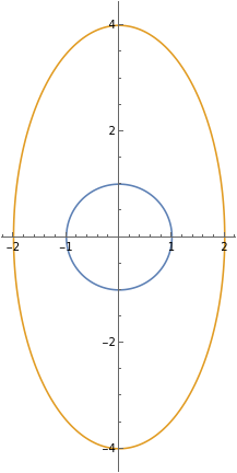

An example. — Figure 5.7.9. An example of curves $C_{1}$ and $K .$

We let

D_{1}

be the region bounded by the two closed curves

C_{1}

and

K,

and we give

D_{1}

a canonical orientation. By definition, the origin is not in

D_{1},

D_{1} \subset U

and the one-form is well defined on

D_{1} .

We can then apply Green's theorem. The boundary of

D_{1}

has two components,

\partial D_{1} = C_{1} \cup K,

and if

D_{1}

is oriented counterclockwise, then the induced orientation on the boundary is counterclockwise for the outer boundary

C_{1}

and clockwise for the inner boundary

K .

To clarify the notation, we write

(C_{1})_{+}

for

C_{1}

with counterclockwise orientation,

K_{+}

for

K

with counterclockwise orientation, and

K_{-}

for

K

with clockwise orientation. So we can write the oriented boundary of

D_{1}

\partial D_{1} = (C_{1})_{+} \cup K_{-} .

By Green's theorem, we have:

\begin{aligned} \int_{D_{1}} d η = & \int_{\partial D_{1}} η \\ = & \int_{(C_{1})_{+}} η + \int_{K_{-}} η \\ = & \int_{(C_{1})_{+}} η - \int_{K_{+}} η, \end{aligned}

where we used the fact that line integrals pick a sign if we change the orientation. But the left-hand-side of the above equation is necessarily zero, since $d η = 0 .$ Therefore,

\int_{(C_{1})_{+}} η = \int_{K_{+}} η,

which is the statement that we were trying to prove, with both curves canonically oriented.

(d) The power of what we did in (c) is to replace the evaluation of the line integral of $η$ along an arbitrary simple closed curve $C_{1}$ that encloses the origin by the evaluation of the line integral of $η$ along a circle $K$ centered at the origin of a certain non-zero radius. But we can evaluate the latter explicitly! Indeed, if $K$ has radius $R,$ for some $R \in R_{> 0},$ then we can parametrize $K$ by $α : [0, 2 π] \to R^{2}$ with

α (θ) = (R \cos (θ), R \sin (θ)) .

The pullback of $η$ is

\begin{aligned} α^{*} η = & \frac{1}{R^{2}} (- R \sin (θ) (- R \sin (θ)) + R \cos (θ) (R \cos (θ))) d θ \\ = & d θ . \end{aligned}

Therefore,

\begin{aligned} \int_{α} η = & \int_{[0, 2 π]} α^{*} η \\ = & \int_{0}^{2 π} d θ \\ = & 2 π . \end{aligned}

So the line integral of $η$ along any circle $K$ centered at the origin is always non-zero and equal to $2 π .$ By (c), we thus conclude that

\int_{C_{1}} η = 2 π

for arbitrary simple closed curves $C_{1}$ that enclose the origin. Very powerful result!