Chapter 3 Limits and continuity

Section 3.1 Motivation

An average rate of accumulation calculation can be useful, but it doesn’t tell you what was happening at any given moment. For example, if you leave an empty container outside over night and it collects some amount of rain water, dividing volume by time to get the average rate of accumulation of the amount of liquid in the container doesn’t tell you whether there was a steady drizzle all night or a sudden downpour for a few minutes at some point. To determine how things were changing instant to instant, we need to measure over much smaller time intervals.
But how “small” is a small enough time interval? For rainfall, maybe second to second. If you are measuring the movement of electrons, a second is still much too large of a time interval.
To get around this problem, in theory we decide that no time interval is small enough to measure instantaneous rate of accumulation. We try to predict the result if we were able to measure average rates of change over smaller and smaller time intervals, forever. The result of this prediction process is called a limit.

Example 3.1.1. Limit of average rate of accumulation calculations.

Suppose we have some quantity modelled by \(q(t) = t^3 \text{,}\) with \(t \) in seconds. How fast is the quantity changing at the instant \(t = 1 \text{?}\) To answer, we compute average rates of change over shorter and shorter time intervals around \(t = 1 \text{,}\) and look for a pattern.
\begin{align*} 0 \amp \le t \le 2 \amp \slope{q}{t} \amp = \frac{2^3 - 0^3 }{2 - 0 } = 4 \\ 0.9 \amp \le t \le 1.1 \amp \slope{q}{t} \amp = \frac{{1.1}^3 - {0.9}^3 }{1.1 - 0.9 } = 3.01 \\ 0.99 \amp \le t \le 1.01 \amp \slope{q}{t} \amp = \frac{{1.01}^3 - {0.99}^3 }{1.01 - 0.99 } = 3.0001 \\ 0.999 \amp \le t \le 1.001 \amp \slope{q}{t} \amp = \frac{{1.001}^3 - {0.999}^3}{1.001 - 0.999} = 3.000001 \end{align*}
If we imagine continuing this process forever, it seems like the average rate of accumulation results will continually get closer to \(3 \text{.}\) We call this value the limit of the process, and can think of it as the instantaneous rate of accumulation at the instant \(t = 1 \text{.}\)
In Example 3.1.1, we considered a limiting process for successive average rate calculations. Each average rate calculation had the same form: we compared a data point a little after \(t = 1 \) with a data point a little before \(t = 1 \text{.}\) That is, we computed the average rate \(\inlineslope{q}{t} \) over the time domain \(1 - h \le t \le 1 + h \text{,}\) where first \(h \) was \(1 \text{,}\) then \(0.1 \text{,}\) then \(0.01 \text{,}\) and so on. So really the limiting process was carried out on the function
\begin{equation*} AV(h) = \slope{q}{t} = \frac{(1 + h)^3 - (1 - h)^3}{(1 + h) - (1 - h)} \end{equation*}
for smaller and smaller values of \(h \text{,}\) where we have named this function \(AV \) to stand for AVerage rate of accumulation. Our conclusion could be expressed as saying
\begin{equation*} AV(h) \approx 3 \end{equation*}
is always true for
\begin{equation*} h \approx 0 \text{.} \end{equation*}
Note that we can’t actually compute \(AV(0) \text{,}\) however, since that would involve division by \(0 \text{.}\)
In the rest of this chapter, we will investigate a limiting process for arbitrary functions, and return to the pattern of a limiting process for average rate of accumulation in Chapter 5.

Section 3.2 Definition and first examples

Motivated by Example 3.1.1, a limiting process tries to answer the following question for a function \(f(t) \) and a specific point \(t = c \text{:}\) Is there some particular value \(L \) so that
\begin{equation*} f(t) \approx L \end{equation*}
is always true for
\begin{equation*} t \approx c \qquad \text{but} \qquad t \neq c \text{?} \end{equation*}
In answering this question, we have to take care with what “approximately equal to \(L \)” and “approximately equal to \(t_0 \)” mean.

Definition 3.2.1. Limit of a function.

We write
\begin{equation*} f(t) \to L \qquad \text{as} \qquad t \to c \end{equation*}
or
\begin{equation*} \lim_{t \to c} f(t) = L \end{equation*}
if values of \(f(t) \) can be made arbitrarily close to \(L \) for all \(t \) sufficiently close to \(c \) but not equal to \(c \text{.}\) If there is no such value \(L \text{,}\) then we say the limit doesn’t exist.

Remark 3.2.2. Limits measure “nearby” behaviour.

If \(t = c \) is in the domain of \(f(t) \text{,}\) we can easily answer the question of what \(f \) is doing at \(t = c \) by just evaluating \(f(c) \text{.}\) The limit instead tries to measure if there is any pattern to the output values of \(f(t) \) for input values that are close (but not equal) to \(c \text{,}\) and the two are not necessarily always the same.

Example 3.2.3. Limit of a square function.

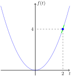
For \(f(t) = t^2 \text{,}\) we have
\begin{equation*} \lim_{t \to 2} f(t) = 4\text{,} \end{equation*}
since clearly \(t^2 \approx 4 \) is true for all \(t \approx 2 \text{.}\)
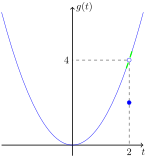
A graph demonstrating that for the square function, output values remain near 4 when input values are taken near 2.
Figure 3.2.4. For the square function, output values remain near \(4 \) when input values are taken near \(2 \text{.}\)

Example 3.2.5. Limit of a modified square function.

Now consider the function
\begin{equation*} g(t) = \begin{cases} t^2, \amp t \neq 2 \\ 2, \amp t = 2 \end{cases} \text{.} \end{equation*}
In this case, we still have
\begin{equation*} \lim_{t \to 2} g(t) = 4\text{,} \end{equation*}
because when we consider \(t \approx 2 \) but \(t \neq 2 \text{,}\) the piecewise definition says that we should use the formula \(g(t) = t^2 \text{.}\) And \(t^2 \approx 4 \) is still true for all \(t \approx 2 \text{.}\)
A graph demonstrating that for a modified square function, output values remain near 4 when input values are taken near 2.
Figure 3.2.6. For a modified square function, output values remain near \(4 \) when input values are taken near \(2 \text{.}\)

Warning 3.2.7. Value at \(t = c \) is irrelevant to the limit.

In both Example 3.2.3 and Example 3.2.5, the limit value exists, but in the first case we found
\begin{equation*} \lim_{t \to 2} f(t) = f(2) \end{equation*}
whereas in the second case we found
\begin{equation*} \lim_{t \to 2} g(t) \neq g(2) \text{.} \end{equation*}

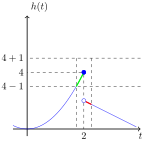
Example 3.2.8. A limit that doesn’t exist.

Now consider the function
\begin{equation*} h(t) = \begin{cases} t^2, \amp t \le 2 \\ 4 - t, \amp t \gt 2 \end{cases} \text{.} \end{equation*}
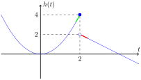
A graph of a piecewise function where not all output values remain near a particular value for inputs near 2.
Figure 3.2.9. Output values for this piecewise function do not stay close to one particular value for \(t \approx 2 \text{.}\)
In Figure 3.2.9, we see that
\begin{equation*} h(t) \approx 4 \end{equation*}
is true for some values of \(t \) close to \(2 \) (in green), while
\begin{equation*} h(t) \approx 2 \end{equation*}
is true for other values of \(t \) close to \(2 \) (in red). Since there is no one value \(L \) so that
\begin{equation*} h(t) \approx L \end{equation*}
is always true for all values of \(t \) close (but not equal) to \(2 \text{,}\) we say that
\begin{equation*} \lim_{t \to 2} h(t) \end{equation*}
does not exist.
What is meant by arbitrarily close and sufficiently close in Definition 3.2.1? It means that no matter how close we mean by “close to \(L \text{,}\)” there is a way to define “close to \(c \)” so that it will indeed be the case that
\begin{equation*} f(t) \approx L \end{equation*}
is true for all
\begin{equation*} t \approx c \qquad\text{but}\qquad t \neq c \text{.} \end{equation*}

Example 3.2.10. Testing the definition of limit.

Let’s revisit
\begin{equation*} \lim_{t \to 2} t^2 = 4 \end{equation*}
from Example 3.2.3, where \(L = 4 \) and \(c = 2 \text{.}\)
  • If we take “close to \(L \)” to mean “within \(1 \) unit of \(L = 4 \)”, then
    \begin{equation*} f(t) \approx 4 \end{equation*}
    is true for all
    \begin{equation*} \sqrt{3} \le t \le \sqrt{5} \text{,} \end{equation*}
    excluding \(t = 2 \text{.}\)
  • If we take “close to \(L \)” to mean “within \(0.1 \) units of \(L = 4 \)”, then
    \begin{equation*} f(t) \approx 4 \end{equation*}
    is true for all
    \begin{equation*} \sqrt{3.9} \le t \le \sqrt{4.1} \text{,} \end{equation*}
    excluding \(t = 2 \text{.}\)
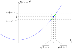
  • If we take “close to \(L \)” to mean “within \(\epsilon \) units of \(L = 4 \)”, where \(\epsilon \) is the smallest (positive) number you can think of, then
    \begin{equation*} f(t) \approx 4 \end{equation*}
    is true for all
    \begin{equation*} \sqrt{4 - \epsilon} \le t \le \sqrt{4 + \epsilon} \text{,} \end{equation*}
    excluding \(t = 2 \text{.}\)
A graph demonstrating that when the limit exists, outputs can be restricted to remain arbitrarily close to the limiting value as long as inputs are restricted to being sufficiently close around the input point of interest.
Figure 3.2.11. When the limit exists, outputs can be restricted to remain arbitrarily close to the limiting value as long as inputs are restricted to being sufficiently close around the input point of interest.

Example 3.2.12. Verifying that a proposed limit value is incorrect.

Now let’s revisit the
\begin{equation*} \lim_{t \to 2} h(t) \end{equation*}
for
\begin{equation*} h(t) = \begin{cases} t^2, \amp t \le 2 \\ 4 - t, \amp t \gt 2 \end{cases} \end{equation*}
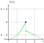
from Example 3.2.8. Suppose we think the limit value is \(4 \text{,}\) since \(h(2) = 4 \text{.}\) If we are generous with our definition of “close to \(L = 4 \)” and take it to mean “within \(3 \) units of \(L = 4 \)”, then yes,
\begin{equation*} h(t) \approx 4 \end{equation*}
is true for all
\begin{equation*} 1 \lt t \lt 3 \text{,} \end{equation*}
excluding \(t = 2 \text{.}\) But if we tighten our definition of “close to \(L = 4 \)” and take it to mean “within \(1 \) units of \(L = 4 \)”, then there will always be some \(t \) close to \(2 \) for which \(h(t) \) is approximately \(2 \) instead of \(4 \text{,}\) no matter how “close” we take “\(t \) close to \(2 \)” to mean.
A generous definition of close can be achieved.
(a) It is possible to restrict to the range \(1 \lt h(t) \lt 7 \) by restricting \(t \) to be in the domain \(1 \lt t \lt 3 \text{.}\)
A tighter definition of close cannot be achieved.
(b) It is not possible to restrict to the range \(3 \lt h(t) \lt 5 \text{,}\) no matter how closely we restrict \(t \) around \(2 \text{.}\)
Figure 3.2.13. A generous definition of “close” might be achieved, but a tighter definition of “close” cannot.
Note that similar reasoning can be used to confirm that
\begin{equation*} \lim_{t \to 2} h(t) = 2 \end{equation*}
is also incorrect.

Section 3.3 Limit laws

Limits adhere to the following useful “laws”. We will delay justifying them until Chapter 24, where we will approach function limits more rigorously from the perspective of sequence limits.

Warning 3.3.2.

A limit of a quotient function were both the numerator and denominator limits are \(0 \) is called \(0 / 0\)-form. Neither of the laws involving quotients in Pattern 3.3.1 (Law 6 and Law 7) applies to such a situation. In fact, a \(0 / 0\)-form quotient limit may or may not exist. See Example 3.4.1 for an example of a \(0 / 0\)-form quotient limit that does exist, and Example 3.4.2 for one that does not exist.

Example 3.3.3. Limit of a quadratic function.

Consider
\begin{equation*} \lim_{t \to 2} 3 t^2 - 4 t + 6 \text{.} \end{equation*}
From Example 3.2.3 we have
\begin{equation*} \lim_{t \to 2} t^2 = 4 \text{,} \end{equation*}
so we may apply the Constant multiple law to obtain
\begin{equation*} \lim_{t \to 2} 3 t^2 = 3 \lim_{t \to 2} t^2 = 3 \cdot 4 = 12 \text{.} \end{equation*}
We may also combine the Constant multiple law with the Limit of the independent variable to obtain
\begin{equation*} \lim_{t \to 2} 4 t = 4 \lim_{t \to 2} t = 4 \cdot 2 = 8 \text{.} \end{equation*}
Finally, we may combine these preliminary results with the Sum and difference laws and the Limit of a constant function to obtain
\begin{align*} \lim_{t \to 2} 3 t^2 - 4 t + 6 \amp = \lim_{t \to 2} 3 t^2 - \lim_{t \to 2} 4 t + \lim_{t \to 2} 6\\ \amp = 12 - 8 + 6 \\ \amp = 10 \text{.} \end{align*}

Example 3.3.4. Limit of a rational function.

Consider
\begin{equation*} \lim_{t \to 2} \frac{(3 t^2 - 4 t + 6) (2 t + 5)}{t^2 - 6} \text{.} \end{equation*}
We have already computed the limit of one of the numerator factors in Example 3.3.3. The limits of the other numerator factor and of the denominator can be calculated similarly:
\begin{align*} \lim_{t \to 2} 2 t + 5 \amp = \lim_{t \to 2} 2 t + \lim_{t \to 2} 5 \amp \lim_{t \to 2} t^2 - 6 \amp = \lim_{t \to 2} t^2 - \lim_{t \to 2} 6\\ \amp = \left(2 \lim_{t \to 2} t\right) + 5 \amp \amp = 4 - 6\\ \amp = 2 \cdot 2 + 5 \amp \amp = -2 \text{.}\\ \amp = 9 \text{,} \end{align*}
We can combine the results of the limits of the two numerator factors using the Product law:
\begin{equation*} \lim_{t \to 2} (3 t^2 - 4 t + 6) (2 t + 5) = 10 \cdot 9 = 90 \text{.} \end{equation*}
Finally, since the denominator limit is nonzero, the Product law applies to yield
\begin{equation*} \lim_{t \to 2} \frac{(3 t^2 - 4 t + 6) (2 t + 5)}{t^2 - 6} = \frac{90}{-2} = -45\text{.} \end{equation*}

Warning 3.3.5. Evaluation of a limit is not just evaluation of the function.

In both Example 3.3.3 and Example 3.3.4, it would appear that the limit results can be obtained simply by evaluating the functions. However, we emphasize again that in general the value of \(f(c) \) is irrelevant to the limit of \(f(t) \) as \(t \to c \).
The situation where the function value \(f(c) \) and the limit value of \(f(t) \) as \(t \to c \) turn out to be the same is a special one that we will give a name to later in this chapter (Section 3.5).

Section 3.4 Computing limits algebraically

A numerical approach like the one used in Example 3.1.1 is good to get an idea of what the value of a limit might be, but an algebraic approach is preferred as it usually leaves no doubt as to the limit value. A particular form of limit that we will want to be able to compute is called 0/0 form, as that is the result if we just try to evaluate with \(t = c \) instead of considering \(t \approx c \) but \(t \neq c \text{.}\)

Example 3.4.1. Pre-cancelling zeros.

Consider
\begin{equation*} \lim_{t \to 1} \frac{t^2 - 1}{t - 1} \text{.} \end{equation*}
If we just consider \(t \approx 1 \text{,}\) then also \(t^2 \approx 1 \text{,}\) which leads to
\begin{align*} t^2 - 1 \amp \approx 0 \amp t - 1 \amp \approx 0 \text{.} \end{align*}
This gives us
\begin{equation*} \frac{t^2 - 1}{t - 1} \approx \frac{0}{0} \text{,} \end{equation*}
which makes no sense. Instead, let’s manipulate the function algebraically first:
\begin{align*} \frac{t^2 - 1}{t - 1} \amp = \frac{(t - 1) (t + 1)}{t - 1} \\ \amp = \frac{\bcancel{(t - 1)} (t + 1)}{\bcancel{t - 1}} \\ \amp = t + 1 \text{.} \end{align*}
Now we can say that
\begin{equation*} \frac{t^2 - 1}{t - 1} = t + 1 \approx 2 \end{equation*}
whenever \(t \approx 1 \) but \(t \neq 1 \text{,}\) so
\begin{equation*} \lim_{t \to 1} \frac{t^2 - 1}{t - 1} = 2\text{.} \end{equation*}
Note that the assumption \(t \neq 1 \) is critical to the algebra. If \(t = 1 \) were part of our consideration, then the cancellation step in the algebra above would actually be performing
\begin{equation*} \frac{\bcancel{0}}{\bcancel{0}} = 1 \text{,} \end{equation*}
which makes no sense.

Example 3.4.2. Not enough zeros to cancel.

Consider
\begin{equation*} \lim_{t \to 1} \frac{t^2 - 1}{{(t - 1)}^2} \text{.} \end{equation*}
Similar to Example 3.4.1, both the numerator and denominator functions are approaching \(0 \) as \(t \to 1 \text{.}\) Again, we’ll first attempt some algebraical manipulation:
\begin{align*} \frac{t^2 - 1}{{(t - 1)}^2} \amp = \frac{(t - 1) (t + 1)}{(t - 1) (t - 1)} \\ \amp = \frac{\bcancel{(t - 1)} (t + 1)}{\bcancel{(t - 1)} (t - 1)} \\ \amp = \frac{t + 1}{t - 1} \text{.} \end{align*}
Now we can say that
\begin{equation*} \frac{t^2 - 1}{{(t - 1)}^2} = \frac{t + 1}{t - 1} \end{equation*}
for all \(t \approx 1 \) but \(t \neq 1 \text{.}\) But now our simplified numerator and denominator functions satisfy
\begin{align*} t + 1 \amp \to 2 \text{,} \amp t - 1 \amp \to 0 \end{align*}
as \(t \to 1 \text{.}\) This puts us in the situation of Law 7 of Pattern 3.3.1, which says that the limit does not exist.

Example 3.4.3. Rationalizing.

Consider
\begin{equation*} \lim_{t \to 1} \frac{\sqrt{t} - 1}{t - 1} \text{.} \end{equation*}
Again, immediately considering \(t \approx 1 \) leads to \(0/0 \) form:
\begin{equation*} \frac{\sqrt{t} - 1}{t - 1} \approx \frac{0}{0} \text{.} \end{equation*}
As this does not tell us the limit value (if any), we need to try to manipulate algebraically. The problem is the pesky square root in the numerator. However, we can rationalize the numerator by multiplying by its conjugate.
\begin{align*} \frac{\sqrt{t} - 1}{t - 1} \amp = \frac{\sqrt{t} - 1}{t - 1} \cdot \frac{\sqrt{t} + 1}{\sqrt{t} + 1} \\ \amp = \frac{(\sqrt{t} - 1)(\sqrt{t} + 1)}{(t - 1)(\sqrt{t} + 1)} \\ \amp = \frac{{(\sqrt{t})}^2 - 1^2}{(t - 1)(\sqrt{t} + 1)} \\ \amp = \frac{\bcancel{t - 1}}{\bcancel{(t - 1)}(\sqrt{t} + 1)} \\ \amp = \frac{1}{\sqrt{t} + 1} \\ \amp \approx \frac{1}{2} \end{align*}
when \(t \approx 1 \) but \(t \neq 1 \text{.}\) In the first step of the algebra above, we are effectively multiplying by \(1 \text{.}\) But we have chosen this particular version of multiplying by \(1 \) so that when we expand the new numerator we get a difference of squares as a result.
From the algebra above, we can conclude that
\begin{equation*} \lim_{t \to 1} \frac{\sqrt{t} - 1}{t - 1} = \frac{1}{2} \text{.} \end{equation*}
Since becoming proficient limit evaluators is not a goal of this course, we leave further examples to the further development of the limiting process applied to average rate of accumulation expressions in Chapter 5.

Section 3.5 Continuous functions

Subsection 3.5.1 Basics

The graphs in Figure 2.3.5 and Figure 2.3.7 have an odd feature — they approach one value then suddenly jump to a different value. We’ll call this type of feature a point of discontinuity. We can detect this kind of behaviour by comparing a functions behaviour near a particular input value (using a limit) to its behaviour at that input value (by evaluation). A function is continuous when these two behaviours agree, and discontinuous when they disagree.

Definition 3.5.1. Continuous at a point.

A function \(f(t) \) is said to be continuous at a specific input value \(t = c \) if the limit of \(f(t) \) as \(t \to c \) exists and satisfies
\begin{equation*} \lim_{t \to c} f(t) = f(c) \text{.} \end{equation*}
Otherwise, the function is said to be discontinuous at that point.

Example 3.5.2.

The calculation in Example 3.2.3 verifies that \(f(t) = t^2 \) is continuous at \(t = 2 \text{,}\) since we had
\begin{equation*} \lim_{t \to 2} f(t) = 4 = f(2) \text{.} \end{equation*}

Example 3.5.3.

The calculation in Example 3.2.5 verifies that the modified square function
\begin{equation*} g(t) = \begin{cases} t^2, \amp t \neq 2 \\ 2, \amp t = 2 \end{cases} \end{equation*}
is discontinuous at \(t = 2 \text{,}\) since we had
\begin{equation*} \lim_{t \to 2} g(t) = 4 \neq g(2) \text{.} \end{equation*}

Example 3.5.4.

The calculation in Example 3.2.8 verifies that the piecewise function
\begin{equation*} h(t) = \begin{cases} t^2, \amp t \le 2 \\ 4 - t, \amp t \gt 2 \end{cases} \end{equation*}
is discontinuous at \(t = 2 \text{.}\) Since we decided that
\begin{equation*} \lim_{t \to 2} h(t) \end{equation*}
does not exist, it is not possible for
\begin{equation*} \lim_{t \to 2} h(t) = h(2) \end{equation*}
to be true as we cannot compare the number \(h(2) \) to a non-existent number.
Graphically, we think of a function as being continuous at an input value \(t = c \) if its graph “flows continuously through” the point \(\bbrac{c, f(c)} \text{,}\) while the graph near a point of discontinuity features some sort of gap or jump. In particular, as noted in Pattern 3.5.5, a function will always be discontinuous at a point that is not in its domain.
Discussing continuity point-by-point is tedious; we generally just look for likely spots for discontinuities. (See below for examples.) Between discontinuities, we make a blanket pronouncement of continuity.

Definition 3.5.6. Continuous on a subdomain.

A function \(f(t) \) is said to be continuous on a specific subdomain if it is continuous at every point in that subdomain.
If a function is continuous on its entire domain we will say exactly that: the function is continuous on its domain. If we just say that a function is continuous, we mean that the function is continuous at all real input values.

Subsection 3.5.2 Types of discontinuities

We will encounter three basic types of discontinuities.

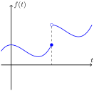
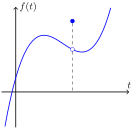
Jump discontinuities.

This occurs when a function suddenly jumps in value, hence the name.
A piecewise function with a jump discontinuity.
(a) A piecewise function can often (but not always!) jump values at transition points.
A function with a redefined point creating a jump discontinuity.
(b) Sometimes the output of a function at one specific input location is specially defined, creating a jump discontinuity.
Figure 3.5.7. Two examples of jump discontinuities.

Removable discontinuities.

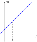
You might think of this kind of discontinuity as a “hole in the graph”. For example, for the function
\begin{equation*} f(t) = \frac{t^2 - 1}{t - 1} \text{,} \end{equation*}
for most values of \(t \) we can simplify the input-output formula to
\begin{equation*} f(t) = \frac{t^2 - 1}{t - 1} = t + 1 \text{,} \end{equation*}
just as we did in Example 3.4.1. This result says that the function’s graph is essentially a line. But as noted in that example, the algebra that led to this simplified formula is not valid for \(t = 1 \text{.}\) Our function is actually undefined at \(t = 1 \text{,}\) and its graph just has a hole there.
A graph with a discontinuity caused by an undefined value.
Figure 3.5.8. A graph with a discontinuity caused by an undefined value.
Why not just define \(f(t) = t + 1 \) in the first place? Our function might be created as the ratio of two other quantities, where the numerator is a model for some quantity, the denominator is a model for a separate quantity, and we want the function to track their ratio. In this case, it is important to record that the ratio is undefined when the second quantity is zero.
However, the fact that \(f(t) = t + 1 \) is true for “almost all” input values justifies the terminology removable discontinuity — we could “remove” the discontinuity by replacing \(f(t) \) by the continuous function \(g(t) = t + 1 \text{,}\) so that \(g(t) = f(t) \) is true for “almost all” input values. Thus \(g \) “fixes” the discontinuity in \(f \text{,}\) and so is called a continuous extension of \(f \text{.}\)

Singularities.

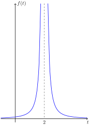
Some functions have a different kind of hole in their domain, near which the function values “explode”.
A graph of a function with a discontinuity caused by a singularity.
Figure 3.5.9. The graph of \(f(t) = 1/(t - 2)^2 \text{,}\) with a singularity at \(t = 2 \text{.}\)
We will call such an input location a singularity for the function. The vertical line at that location (as represented by a dashed line in the example graph in Figure 3.5.9) is called a vertical asymptote for the function’s graph.
We will study singularities and vertical asymptotes more in Chapter 4.

Subsection 3.5.3 The Intermediate Value Theorem

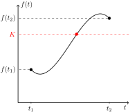
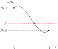
An important feature of continuous graphs is that they cannot “skip over” any particular output level.
A continuous function ascending through all possible output values from low to high.
The graph of a function over a closed, bounded domain \(t_1 \lt t \lt t_2 \) is drawn on a set of \(tq \)-axes. The graph begins at a closed endpoint at position \(\bbrac{t_1, f(t_1)} \text{.}\) From there is dips slightly down to a trough before rising significantly up to a peak, before dipping slightly again down to a closed endpoint at position \(\bbrac{t_2, f(t_2)} \text{.}\) In this configuration, \(f(t_1) \lt f(t_2) \text{.}\) The values \(q = f(t_1) \) and \(q = f(t_2) \) are marked on the vertical axis, and a dashed horizontal line runs from each of those positions on the vertical axis to the corresponding endpoint of the graph.
A value \(q = K \) is marked on the vertical axis, approximately three-quarters of the way from \(q = f(t_1) \) up to \(q = f(t_2) \text{,}\) and a third dashed horizontal line runs from this position on the vertical axis to the right edge of the view. This horizontal line necessarily intersects the graph, and the point of intersection is marked on the graph to illustrate the conclusion of the Theorem 3.5.10 in this case.
(a) Ascending through each possible output value.
A continuous function descending through all possible output values from high to low.
The graph of a function over a closed, bounded domain \(t_1 \lt t \lt t_2 \) is drawn on a set of \(tq \)-axes. The graph begins at a closed endpoint at position \(\bbrac{t_1, f(t_1)} \text{.}\) From there is rises slightly up to a peak before descending significantly down to a trough, before rising slightly again up to a closed endpoint at position \(\bbrac{t_2, f(t_2)} \text{.}\) In this configuration, \(f(t_1) \gt f(t_2) \text{.}\) The values \(q = f(t_1) \) and \(q = f(t_2) \) are marked on the vertical axis, and a dashed horizontal line runs from each of those positions on the vertical axis to the corresponding endpoint of the graph.
A value \(q = K \) is marked on the vertical axis, approximately three-quarters of the way from \(q = f(t_1) \) down to \(q = f(t_2) \text{,}\) and a third dashed horizontal line runs from this position on the vertical axis to the right edge of the view. This horizontal line necessarily intersects the graph, and the point of intersection is marked on the graph to illustrate the conclusion of the Theorem 3.5.10 in this case.
(b) Descending through each possible output value.
Figure 3.5.11. As a continuous function ascends/descends, it must take on all possible output values between initial and final output values.

Example 3.5.12. Searching for horizontal intercepts.

The graph of the cubic function
\begin{equation*} p(t) = 5 - t + t^2 - t^3 \end{equation*}
is continuous, so from the information
\begin{align*} p(1) \amp = 4 \text{,} \amp p(2) \amp = -1 \end{align*}
we may conclude that the graph must descend through every possible output value between \(4 \) and \(-1 \) over the domain \(1 \le t \le 2 \text{.}\) (Note, however, that this doesn’t mean the graph cannot ascend on some portion of this domain.)
In particular, since \(p(1) \gt 0 \) and \(p(2) \lt 0 \text{,}\) we may apply the Intermediate Value Theorem with \(K = 0 \) to conclude that there must be at least one solution to
\begin{equation*} 5 - t + t^2 - t^3 = 0 \end{equation*}
somewhere between \(t = 1 \) and \(t = 2 \text{.}\)