Klein-Gordon Equation in Schrödinger Form

For some calculations it is useful to write the Klein-Gordon equation in the two-component form

$$\chi_1 = \frac{1}{2} \left[ \phi + \frac{i}{m} \left(\partial^0 + ieA^0\right)\phi\right] ,$$ (4.84)

$$\chi_2 = \frac{1}{2} \left[ \phi - \frac{i}{m} \left(\partial^0 + ieA^0\right)\phi\right] .$$ (4.85)

We see that $\phi = \chi_1 + \chi_2$ and $\chi_1 - \chi_2 = \frac{i}{m}\left(\partial^0+ieA^0\right)\phi$.

The charge density for these state is (setting $\hbar = c = 1$)

$$\rho = \frac{ie}{2m} \left[ \phi^*(\partial^0 + ieA^0)\phi - \phi(\partial^0 - ieA^0)\phi^* \right] ,$$

$$= \frac{ie}{2m} \frac{m}{i} [(\chi_1+\chi_2)^*(\chi_1-\chi_2) + (\chi_1+\chi_2)(\chi_1-\chi_2)^*] ,$$

$$= \frac{e}{2} \left( \chi_1^*\chi_1 - \chi_2^*\chi_2 + \chi_1^*\chi_1 - \chi_2^*\chi_2 \right) ,$$

$$= e \left( \vert\chi_1\vert^2 - \vert\chi_2\vert^2 \right) ,$$ (4.86)

which is rather simple and somewhat similar to the nonrelativistic case.

$\chi_1, \chi_2$ obey the coupled equation

$$(i\partial^0 -eA^0)\chi_1 = \frac{1}{2} \left(i\partial^0 - eA^0\right)\phi + \frac{i}{2m} \left(i\partial^0 - eA^0\right)\left(\partial^0 + ieA^0\right)\phi ,$$

$$= \frac{m}{2} (\chi_1-\chi_2) + \frac{1}{2m} \left(i\partial^0-eA^0\right)^2\phi ,$$

$$= \frac{m}{2} (\chi_1-\chi_2) + \frac{1}{2m} \left[\left(-i\vec{\nabla} - e\vec{A}\right)^2 + m^2\right](\chi_1+\chi_2) ,$$

$$= \frac{1}{2m} \left(-i\vec{\nabla} - e\vec{A}\right)^2(\chi_1+\chi_2) + m\chi_1 ,$$ (4.87)

and

$$(i\partial^0 -eA^0)\chi_2 = \frac{m}{2} \left(\chi_1 - \chi_2\right) - \frac{1}{2m} \left[\left(-i\vec{\nabla} -e\vec{A}\right)^2 +m^2\right] \left(\chi_1 + \chi_2\right) ,$$

$$= -\frac{1}{2m} \left(-i\vec{\nabla} -e\vec{A}\right)^2 \left(\chi_1+\chi_2\right) - m\chi_2 .$$ (4.88)

If we define the 2-component spinor

$$\chi = \left( \begin{array}{c} \chi_1 \\ \chi_2 \end{array}\right)$$ (4.89)

we can combine equations 4.87 and 4.88 to be

$$\left( i\partial^0 - eA^0 \right) \left( \begin{array}{c} \c... ...\left( \begin{array}{r} \chi_1 \\ -\chi_2 \end{array}\right) ,$$ (4.90)

$$\left( i\partial^0 - eA^0 \right) \left( \begin{array}{cc} 1 & 0 ... ...{array} \right) \left( \begin{array}{c} \chi_1 , \\ \chi_2 \end{array} \right) = \frac{1}{2m} \left( -i\vec{\nabla} - e\vec{A} \right)^2 \left( \b... ...nd{array} \right) \left( \begin{array}{c} \chi_1 \\ \chi_2 \end{array} \right)$$

$$+ m \left( \begin{array}{cc} 1 & 0 \\ 0 & -1 \end{array} \right) \left( \begin{array}{c} \chi_1 \\ \chi_2 \end{array}\right) .$$ (4.91)

Using the Pauli matrices, $\vec{\tau}$,

$$\tau_3 + i\tau_2 = \left( \begin{array}{rr} 1 & 1 \\ -1 & -1 \end{array} \right)$$ (4.92)

and we can write

$$(i\partial^0 - eA^0)\chi = \left[ \frac{1}{2m} (-i\vec{\nabla} - e\vec{A})^2(\tau_3 + i\tau_2) + m\tau_3 \right] \chi .$$ (4.93)

This is a first order Schrödinger equation (cf. $\partial^0\chi = H\chi$). The quantity in square brackets is $H - eA^0$.

Also in this notation, the charge density can be written as

$$\rho = e (\vert\chi_1\vert^2 - \vert\chi_2\vert^2) = e \chi^\dagger \tau_3 \chi .$$ (4.94)

The normalization condition becomes

$$\langle\chi\vert\chi\rangle = \int d^3x\chi^\dagger(x)\tau_3\chi(x) = \pm 1 .$$ (4.95)

It will be shown later that the sign is determined by whether we start with particles ($+$) or antiparticles ($-$).

The Klein-Gordon Hamiltonian is

$$H = \frac{1}{2m} (-i\vec{\nabla} - e\vec{A})^2 (\tau_3 + i\tau_2) + m\tau_3 + eA^0 .$$ (4.96)

The Hamiltonian appears to be non-hermitian, since

$$(\tau_3 +i\tau_2)^\dagger = \tau_3 -i\tau_2 \ne \tau_3 +i\tau_2 .$$ (4.97)

However

$$\langle\chi^\prime\vert H\vert\chi\rangle = \int d^3x {\chi^\prime}^\dagger (x)\tau_3 H\chi(x)$$ (4.98)

and

$$\langle\chi^\prime\vert H\vert\chi\rangle^* = \left( \int d^3x {\chi^\prime}^\dagger(x) \tau_3 H \chi(x) \right)^\dagger ,$$

$$= \int d^3x \chi^\dagger(x) H^\dagger \tau_3 \chi^\prime(x) ,$$

$$= \int d^3x \chi^\dagger(x) \tau_3 (\tau_3 H^\dagger \tau_3) \chi^\prime(x) ,$$

$$= \langle \chi\vert\tau_3H^\dagger\tau_3\vert\chi^\prime\rangle .$$ (4.99)

We notice that

$$\tau_3(\tau_3 + i\tau_2)^\dagger\tau_3 = \tau_3(\tau_3 - i\tau_2)\tau_3 = \tau_3 -i\tau_3\tau_2\tau_3$$ (4.100)

and

$$\tau_3\tau_2\tau_3 = \left( \begin{array}{rr} 1 & 0 \\ 0 & ... ...gin{array}{rr} 0 & i \\ -i & 0 \end{array} \right) = -\tau_2$$ (4.101)

gives

$$\tau_3(\tau_3 + i\tau_2)^\dagger\tau_3 = \tau_3 + i\tau_2 .$$ (4.102)

Therefore

$$\tau_3 H^\dagger \tau_3 = H .$$ (4.103)

Because of the normalization condition, the Hamiltonian is effectively hermitian.

Consider the free particle solutions

$$\chi_1 = \frac{1}{2} \left[ \phi + \frac{i}{m}\partial^0\phi... ... \frac{1}{2} \left[ \phi - \frac{i}{m}\partial^0\phi \right] .$$ (4.104)

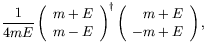
A positive-energy plane-wave solution normalized to unit density (equation 4.41) is

$$\phi(x) = \sqrt{\frac{m}{E}} e^{-i(Et - \vec{p}\cdot\vec{x})} = \sqrt{\frac{m}{E}} e^{-ip\cdot x} .$$ (4.105)

Since $\partial^0\phi = -iE\phi$,

$$\chi_1 = \frac{1}{2}\left(1 + \frac{E}{m}\right)\phi \quad \... ...} \quad \chi_2 = \frac{1}{2}\left(1 - \frac{E}{m}\right)\phi .$$ (4.106)

We can write

$$\chi \equiv \left( \begin{array}{c} \chi_1 \\ \chi_2 \end{ar... ...ht) e^{-ip\cdot x} \equiv \chi^{(+)}(\vec{p}) e^{-ip\cdot x} ,$$ (4.107)

where

$$\chi^{(+)}(\vec{p}) = \frac{1}{2\sqrt{mE}} \left( \begin{array}{c} m+E \\ m-E \end{array} \right) .$$ (4.108)

A corresponding negative-energy plane-wave solution is

$$\phi(x) = \sqrt{\frac{m}{E}} e^{-i(-Et - \vec{p}\cdot\vec{x})}$$ (4.109)

giving

$$\chi^{(-)}(\vec{p}) = \frac{1}{2\sqrt{mE}} \left( \begin{array}{c} m-E \\ m+E \end{array} \right) .$$ (4.110)

Orthogonality shows

$$\langle \chi^{(+)}(\vec{p}) \vert \chi^{(+)}(\vec{p}) \rangle \equiv {\chi^{(+)}}^\dagger(\vec{p}) \tau_3 \chi^{(+)}(\vec{p}) ,$$

$$= \frac{1}{4mE} \left( \begin{array}{r} m+E \\ m-E \end{array}\right)^\dagger \left( \begin{array}{r} m+E \\ -m+E \end{array}\right) ,$$

$$= \frac{1}{4mE} [(m+E)(m+E) + (m-E)(-m+E)] ,$$

$$= \frac{1}{4mE} (m^2 + 2mE + E^2 - m^2 + 2mE - E^2) ,$$

$$= 1 ,$$ (4.111)

and it can also be shown that

$$\langle \chi^{(-)}(\vec{p}) \vert \chi^{(-)}(\vec{p}) \rangle = -1 ,$$ (4.112)

$$\langle \chi^{(+)}(\vec{p}) \vert \chi^{(-)}(\vec{p}) \rangle = 0 ,$$ (4.113)

$$\langle \chi^{(-)}(\vec{p}) \vert \chi^{(+)}(\vec{p}) \rangle = 0 .$$ (4.114)

In the nonrelativistic limit we have

$$E = (p^2 + m^2)^{1/2} = m\left(1 + \frac{p^2}{m^2}\right)^{1... ...(1 + \frac{1}{2}\frac{p^2}{m^2} \right) = m + \frac{p^2}{2m} .$$ (4.115)

The components of equation 4.108 are

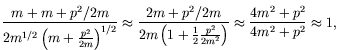$$\frac{m+E}{2\sqrt{mE}} \approx \frac{m+m+p^2/2m}{2m^{1/2}\left(m+\frac{p^2}{2m}\right)^{1/2}} \a... ...rac{1}{2}\frac{p^2}{2m^2}\right)} \approx \frac{4m^2+p^2}{4m^2+p^2} \approx 1 ,$$ (4.116)

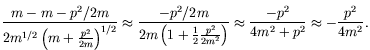$$\frac{m-E}{2\sqrt{mE}} \approx \frac{m-m-p^2/2m}{2m^{1/2}\left(m+\frac{p^2}{2m}\right)^{1/2}} \a... ...rac{p^2}{2m^2}\right)} \approx \frac{-p^2}{4m^2+p^2} \approx -\frac{p^2}{4m^2}.$$ (4.117)

Equation 4.108 in the nonrelativistic limit is

$$\chi^{(+)}(\vec{p}) \approx \left(\begin{array}{c} 1 \\ -p^... ...ht) \approx \left(\begin{array}{c} 1 \\ 0 \end{array}\right) ,$$ (4.118)

which holds to second order in the velocity. Similarly

$$\chi^{(-)}(\vec{p}) \approx \left( \begin{array}{c} 0 \\ 1 \end{array}\right) .$$ (4.119)

By completeness, any wavepacket can be expanded in terms of a linear combination of positive- and negative-energy solutions.

$$\phi(\vec{x},t) = \int \frac{d^3p}{(2\pi)^3} e^{i\vec{p}\cdot\vec{x}} \left[ a^{(+)... ...p}}(t)\chi^{(+)}(\vec{p}) + a^{(-)}_{-\vec{p}}(t)\chi^{(-)}(-\vec{p}) \right] ,$$ (4.120)

$$= \int \frac{d^3p}{(2\pi)^3} \left[ a^{(+)}_{\vec{p}}(t)\chi^{(+)}(... ...} + a^{(-)}_{\vec{p}}(t)\chi^{(-)}(\vec{p}) e^{-i\vec{p}\cdot\vec{x}} \right] ,$$ (4.121)

where $\chi(\vec{p})$ only depends on the magnitude of $\vec{p}$, and $a_{\vec{p}}(t)$ is a function of time and the magnitude of $\vec{p}$.

If the wave function is normalized to unity we have

$$1 \equiv \langle\phi\vert\phi\rangle = \int d^3x \phi^\dagger(\vec{x},t) \tau_3 \phi(\vec{x},t) ,$$

$$= \int d^3x \frac{d^3p^\prime}{(2\pi)^3} \frac{d^3p}{(2\pi)^3} \lef... ...{(-)}}^\dagger(\vec{p}^{\:\prime)} e^{i\vec{p}^{\:\prime}\cdot\vec{x}}] \right.$$

$$\tau_3 \left. [a^{(+)}_{\vec{p}}(t)\chi^{(+)}(\vec{p})e^{i\vec{p}... ...} + a^{(-)}_{\vec{p}}(t)\chi^{(-)}(\vec{p})e^{-i\vec{p}\cdot\vec{x}}] \right] ,$$

$$= \int d^3x \frac{d^3p^\prime}{(2\pi)^3} \frac{d^3p}{(2\pi)^3} [{a^... ...\prime})\tau_3\chi^{(+)}(\vec{p}) e^{i\vec{x}\cdot(\vec{p}-\vec{p}^{\:\prime})}$$

$$+ {a^{(-)}_{\vec{p}}}^*(t)a^{(-)}_{\vec{p}}(t) {\chi^{(-)}}^\dagg... ...prime})\tau_3\chi^{(-)}(\vec{p}) e^{-i\vec{x}\cdot(\vec{p}-\vec{p}^{\:\prime})}$$

$$+ {a^{(+)}_{\vec{p}}}^*(t)a^{(-)}_{\vec{p}}(t) {\chi^{(+)}}^\dagg... ...prime})\tau_3\chi^{(-)}(\vec{p}) e^{-i\vec{x}\cdot(\vec{p}+\vec{p}^{\:\prime})}$$

$$+ {a^{(-)}_{\vec{p}}}^*(t)a^{(+)}_{\vec{p}}(t) {\chi^{(-)}}^\dagg... ...me})\tau_3\chi^{(+)}(\vec{p}) e^{i\vec{x}\cdot(\vec{p}+\vec{p}^{\:\prime})} ] ,$$

$$= \int \frac{d^3p}{(2\pi)^3} \left[ \vert a^{(+)}_{\vec{p}}(t)\vert^2 - \vert a^{(-)}_{\vec{p}}(t)\vert^2 \right] .$$ (4.122)