Electrodynamic processes can be classified by the number and type of particles in the initial state. Our goal in this chapter is to consider the two-particle initial states that led to scattering processes. Photon-electron scattering will be considered in this section, while the photon-photon and electron-electron systems will be consider in subsequent sections. Our use of the word ``electron'' has been generic and includes both electrons and positrons, in general.
The photon-electron system can have two kinds of final states, those in which there is only one electron present (and one or more photons), and those in which there are also one or more electron-positron pairs present. Processes leading to the former kind of final states may be called photon-electron scattering, whereas processes in which pairs are produced can be referred to as pair production in photon-electron collisions.
Photon-electron scattering with only one photon in the final state is
the lowest-order photon-electron process involving a real incident photon.
The separation of the lowest-order from the higher order contributions is
an idealization which does not correspond to physical reality.
In any measurement, the energy of the final state can only be determined
to within the energy resolution of the detector.
It is therefore impossible to determine with certainty whether the final
state contains exactly one photon or whether it contains an additional
number of very soft (low energy) photons.
These multiple-photon final states are suppressed relative to the
lowest-order single-photon final state by at least order ![]() .
.
The lowest order photon-electron scattering process is second-order in
![]() and is called Compton scattering.
The Compton scattering process differs from Bremsstrahlung in that the
incoming photon is real.
Because of charge conjugation invariance of the
and is called Compton scattering.
The Compton scattering process differs from Bremsstrahlung in that the
incoming photon is real.
Because of charge conjugation invariance of the ![]() -matrix, the
cross-section for the photon-electron process is equal to the
cross-section for the photon-positron process.
-matrix, the
cross-section for the photon-electron process is equal to the
cross-section for the photon-positron process.
Figure 7.7 shows the two diagrams leading to Compton scattering. It is important to realize that only the sum of the two diagrams in figure 7.7 describes photon-electron scattering. The separation of a matrix element into terms corresponds to the individual diagrams, though extremely useful, has in general no physical meaning. Only the sum of both diagrams is observable.
In the first diagram (figure 7.7a), the incident photon
(![]() ) is absorbed by the incident electron (
) is absorbed by the incident electron (![]() ) and
then the electron emits a photon (
) and
then the electron emits a photon (
![]() )
into the final state.
In the second diagram (figure 7.7b), the incident electron
(
)
into the final state.
In the second diagram (figure 7.7b), the incident electron
(![]() ) emits a photon (
) emits a photon (
![]() ) before it absorbs
the incident photon (
) before it absorbs
the incident photon (![]() ).
Since each photon is associated with a different momentum four-vector
and each electron path can be labeled as refering to the first, second
or third electrons, we have two distinct Feynman diagrams in
figure 7.7.
The two diagrams are different since they differ in the sequence of the
emitted and absorbed photons as one follows the arrows in the electron
paths.
One can draw the second diagram such that the intermediate electron is
horizontal in the diagram and the two photon do not cross in the
diagram.
This horizontal-electron diagram is not topologically different from the
diagram in figure 7.7b and will not be considered further.
Compton scattering is thus the process
).
Since each photon is associated with a different momentum four-vector
and each electron path can be labeled as refering to the first, second
or third electrons, we have two distinct Feynman diagrams in
figure 7.7.
The two diagrams are different since they differ in the sequence of the
emitted and absorbed photons as one follows the arrows in the electron
paths.
One can draw the second diagram such that the intermediate electron is
horizontal in the diagram and the two photon do not cross in the
diagram.
This horizontal-electron diagram is not topologically different from the
diagram in figure 7.7b and will not be considered further.
Compton scattering is thus the process
![]() , in
which the conservation of energy-momentum requires
, in
which the conservation of energy-momentum requires
![]() .
.
Let ![]() represent an incident photon which is absorbed by an
electron at one vertex and
represent an incident photon which is absorbed by an
electron at one vertex and
![]() represent
a final photon emitted at the second vertex:
represent
a final photon emitted at the second vertex:
| (7.224) |
where ![]() and
and
![]() .
.
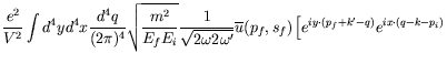
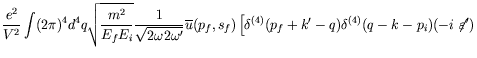
The second-order Compton amplitude is, after carrying out the Fourier transformation to momentum space,
Each term in equation 7.225 represents one of the eight diagrams
shown in figure 7.8.
Not every term that occurs in the scattering amplitude is physically
relevant to the process considered.
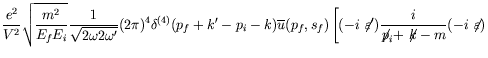
The first two diagrams (figures 7.8a and 7.8b) are
the processes we are interested in when studying Compton scattering.
The second pair of diagrams (figures 7.8c and 7.8d)
have the photon momenta ![]() and
and ![]() interchanged.
This interchange of momenta corresponds to the scattering of an incident
photon with momentum
interchanged.
This interchange of momenta corresponds to the scattering of an incident
photon with momentum ![]() to a final photon with momentum
to a final photon with momentum ![]() .
The process represented by these diagrams is not the physical process
that we are interested in and has energy-momentum conserving conditions
that are incompatible with the process we are interested in.
We thus drop these terms from the scattering amplitude since they are
not the process under study.
The third and fourth pairs of diagrams have two photons in the final
state (figures 7.8e and 7.8f) and two photons in the
initial state (figures 7.8g and 7.8h),
respectively.
These processes are not kinematically allowed.
Such terms in the scattering amplitude contain delta
functions with an argument describing these kinematically forbidden
processes.
The delta functions cause these terms to vanish when the momenta is
integrated over.
.
The process represented by these diagrams is not the physical process
that we are interested in and has energy-momentum conserving conditions
that are incompatible with the process we are interested in.
We thus drop these terms from the scattering amplitude since they are
not the process under study.
The third and fourth pairs of diagrams have two photons in the final
state (figures 7.8e and 7.8f) and two photons in the
initial state (figures 7.8g and 7.8h),
respectively.
These processes are not kinematically allowed.
Such terms in the scattering amplitude contain delta
functions with an argument describing these kinematically forbidden
processes.
The delta functions cause these terms to vanish when the momenta is
integrated over.
For the diagrams we are interested in, we retain from the incident
photon wave function only the first term,
![]() , which
corresponds to absorption at
, which
corresponds to absorption at ![]() of a photon of four-momentum
of a photon of four-momentum ![]() from the radiation field, and retain from the final photon wave function
only the second term,
from the radiation field, and retain from the final photon wave function
only the second term,
![]() , which represents
the emission at
, which represents
the emission at ![]() of a photon with four-momentum
of a photon with four-momentum ![]() .
.
The amplitude now becomes
 |
|||
 |
|||
 |
|||
| (7.226) |
Notice that ![]() is symmetric under interchange of
is symmetric under interchange of ![]() and
and
![]() with
with ![]() and
and
![]() , respectively.
The two diagrams in figure 7.7 are thus related by this
symmetry.
This is known as crossing symmetry, and it persists as an exact
symmetry to all orders in
, respectively.
The two diagrams in figure 7.7 are thus related by this
symmetry.
This is known as crossing symmetry, and it persists as an exact
symmetry to all orders in ![]() .
.
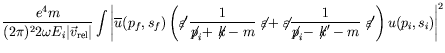
We form the cross-section ![]() by squaring the amplitude, then
dividing by
by squaring the amplitude, then
dividing by
![]() to form a rate per volume.
We then divide the rate by an incident flux
to form a rate per volume.
We then divide the rate by an incident flux
![]() ,
where
,
where
![]() is the relative velocity of the photons
with respect to the electrons.
Then we divide by the number of target particles per unit volume
is the relative velocity of the photons
with respect to the electrons.
Then we divide by the number of target particles per unit volume ![]() .
Finally, summing over phase space of the final particles
.
Finally, summing over phase space of the final particles
![]() ,
, ![]() becomes
becomes
 |
|||
| (7.227) |
where
![]() is the invariant matrix element for Compton
scattering.
It is a function of the four-momenta
is the invariant matrix element for Compton
scattering.
It is a function of the four-momenta ![]() and
and ![]() .
.
We use
![]() to write
the differential cross-section per unit solid angle for scattering
into a differential angular interval between
to write
the differential cross-section per unit solid angle for scattering
into a differential angular interval between ![]() and
and
![]() , and
, and ![]() and
and ![]() .
The integral over all recoil electron momenta can be evaluated with the
aid of the previously developed covariant expression
.
The integral over all recoil electron momenta can be evaluated with the
aid of the previously developed covariant expression
| (7.228) |
The differential cross-section now becomes
| (7.229) |
where the kinematic variables in the matrix element
![]() must
now obey the condition
must
now obey the condition
![]() .
.
The cross-section simplifies considerably if we calculate it in the rest
system of the initial or final electron.
In most experiments the initial electron is practically at rest in the
laboratory so we will work in the rest frame of the initial electron.
In this frame ![]() , the incident beam consists of photons with
unit velocity, such that
, the incident beam consists of photons with
unit velocity, such that
![]() .
The differential cross-section now becomes
.
The differential cross-section now becomes
where ![]() is the angle between the initial and final state photons.
is the angle between the initial and final state photons.
The last line in equation 7.230 was obtained by using the root of
the delta function to relate ![]() to
to ![]() :
:
This is known as the Compton condition.
This kinematic relationship takes on a simple form if one uses the
wavelength,
![]() :
:
| (7.232) |
This is the familiar Compton formula.
The wavelength of the scattered photon is increased by an amount of
order ![]() , and
, and ![]() is called the Compton wavelength.
is called the Compton wavelength.
The differential cross-section for electrons and photons with specific initial and final state polarizations is now
| (7.233) |
We can simplify the spinor matrix element considerably by choosing the special gauge in which both initial and final photons are transversely polarized in the laboratory frame. We choose
| (7.234) | |||
| (7.235) |
Since the electron is initially at rest it follows that
This amounts to choosing the ``radiation gauge'' in which the
electromagnetic potential has no time component.
However, the condition in equation 7.236 can be imposed in any
given frame of reference.
This can be shown by applying a gauge transformation to any arbitrary set
of polarization vectors ![]() and
and
![]() .
The normalization and transversality conditions are not effected by the
transformation.
Thus without restricting the generality of our calculation we will
impose the condition in equation 7.236.
.
The normalization and transversality conditions are not effected by the
transformation.
Thus without restricting the generality of our calculation we will
impose the condition in equation 7.236.
Because of our choice of gauge,
![]() and
and
![]() anticommute
with
anticommute
with
![]() , and
, and
![]() and
and
![]() anticommute
with
anticommute
with
![]() .
The invariant matrix element thus becomes
.
The invariant matrix element thus becomes
| (7.237) |
where the energy-projection operator
![]() has been
used in the last step.
has been
used in the last step.
We now consider the case when the electrons are unpolarized but the
initial and final state photons may be polarized with polarizations
![]() and
and
![]() , respectively.
We thus average over the initial electron spin and sum over the final
electron spin:
, respectively.
We thus average over the initial electron spin and sum over the final
electron spin:
| (7.238) |
Applying the usual trace techniques, we have
| (7.239) |
where we have used the rule
![]() in the last factor.
in the last factor.
There are traces with up to eight ![]() -matrices in them.
To reduce the traces which contain the same vectors, we commute the
-matrices in them.
To reduce the traces which contain the same vectors, we commute the
![]() -matrices until the identical vectors are alongside each other,
then the identity
-matrices until the identical vectors are alongside each other,
then the identity
![]() removes two
removes two ![]() -matrices.
We also make use of
-matrices.
We also make use of ![]() ,
,
![]() ,
,
![]() and
and
![]() .
Evaluating the traces one by one, we have
.
Evaluating the traces one by one, we have
| (7.240) |
Using the symmetry we had earlier
![]() we have
we have
| (7.241) |
We show that the two cross-terms are equal:
| (7.242) |
Using energy-momentum conservation we have
| (7.243) |
Therefore the differential cross-section becomes
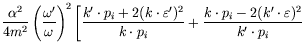 |
|||
![$\displaystyle \frac{\alpha^2}{4m^2}\left(\frac{\omega^\prime}{\omega}\right)^2
...
...
p_i}{k^\prime\cdot p_i} + 4(\varepsilon^\prime\cdot\varepsilon)^2 - 2\right] .$](img4241.png) |
(7.244) |
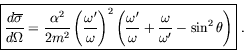
The calculation of the invariant matrix element has so far been covariant. In the rest frame of the initial electron the differential cross-section becomes
![\begin{displaymath}
\fbox{$\displaystyle
\frac{d\overline{\sigma}}{d\Omega}(\lam...
...e} +
4(\varepsilon^\prime\cdot\varepsilon)^2 - 2\right]
$}\ ,
\end{displaymath}](img4242.png) |
(7.245) |
which is the Klein-Nishina formula for Compton scattering.
In the low-energy limit of
![]() , equation 7.231
shows that
, equation 7.231
shows that
![]() and the cross-section
reduces to the classical Thomson scattering
and the cross-section
reduces to the classical Thomson scattering
| (7.246) |
where
| (7.247) |
is the classical electron radius.
For forward scattering,
![]() and according to
equation 7.231
and according to
equation 7.231
![]() .
The Thomson cross-section is thus also valid for forward scattering at all
energies.
.
The Thomson cross-section is thus also valid for forward scattering at all
energies.
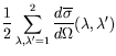
Returning to the general expression for the cross-sections, we can sum
over final-state photon polarizations
![]() and
average over initial-state polarizations
and
average over initial-state polarizations
![]() to obtain
the unpolarized cross-section.
to obtain
the unpolarized cross-section.
 |
|||
![$\displaystyle \frac{\alpha^2}{8m^2} \left(\frac{\omega^\prime}{\omega}\right)^2...
...} +
4(\varepsilon_\lambda\cdot\varepsilon^\prime_{\lambda^\prime})^2 -
2\right]$](img4255.png) |
|||
![$\displaystyle \frac{\alpha^2}{2m^2} \left(\frac{\omega^\prime}{\omega}\right)^2...
...^2
(\varepsilon_\lambda\cdot\varepsilon^\prime_{\lambda^\prime})^2 -
2\right] .$](img4257.png) |
(7.248) |
We can evaluate the remaining spin sum by supposing the incident
photon arrives along the ![]() -direction, while the final photon departs
into the solid angle
-direction, while the final photon departs
into the solid angle ![]() described by polar angles
described by polar angles ![]() and
and
![]() such that
such that
| (7.249) | |||
| (7.250) |
We may select the associated polarization vectors to be
| (7.251) | |||
| (7.252) |
It is easy to show that this choice of vectors satisfies all the required normalization and orthogonality relationships. We obtain
The cross-section thus becomes
 |
(7.254) |
The low-energy for forward-scattering limit (classical limit) now becomes
| (7.255) |
To integrate the differential cross-section, we simplify the notation
by introducing ![]() , and use equation 7.231 to write
, and use equation 7.231 to write
| (7.256) |
To perform the integration, define ![]() , then
, then
| (7.257) |
Using the integrals (![]() is an arbitrary constant)
is an arbitrary constant)
| (7.258) | |||
![$\displaystyle -\left.\frac{1}{2b(1+bx)^2}\right\vert _0^2 =
\frac{1}{2b} \left[ 1 - \frac{1}{(1+2b)^2} \right] ,$](img4287.png) |
(7.259) | ||
| (7.260) | |||
| (7.261) |
we can write
| (7.262) |
which is valid for all initial photon energies ![]() .
.
For low energies,
![]() and
and
| (7.263) |
which is again the classical Thomson cross-section.
At high energies,
![]() and
and
| (7.264) |
![\begin{figure}\begin{center}
\begin{picture}(355,195)(-20,-25)
\SetWidth{0.75}
%...
...{$y$}
\Text(50,-10)[ct]{b)}
\end{picture}}
\end{picture}\end{center}\end{figure}](img4037.png)
![\begin{figure}\begin{center}
\begin{picture}(455,265)(-5,-5)
\SetWidth{0.75}
% n...
...{6}
\Text(45,0)[cb]{g)}
\end{picture}}
\par\end{picture}\end{center}\end{figure}](img4068.png)
