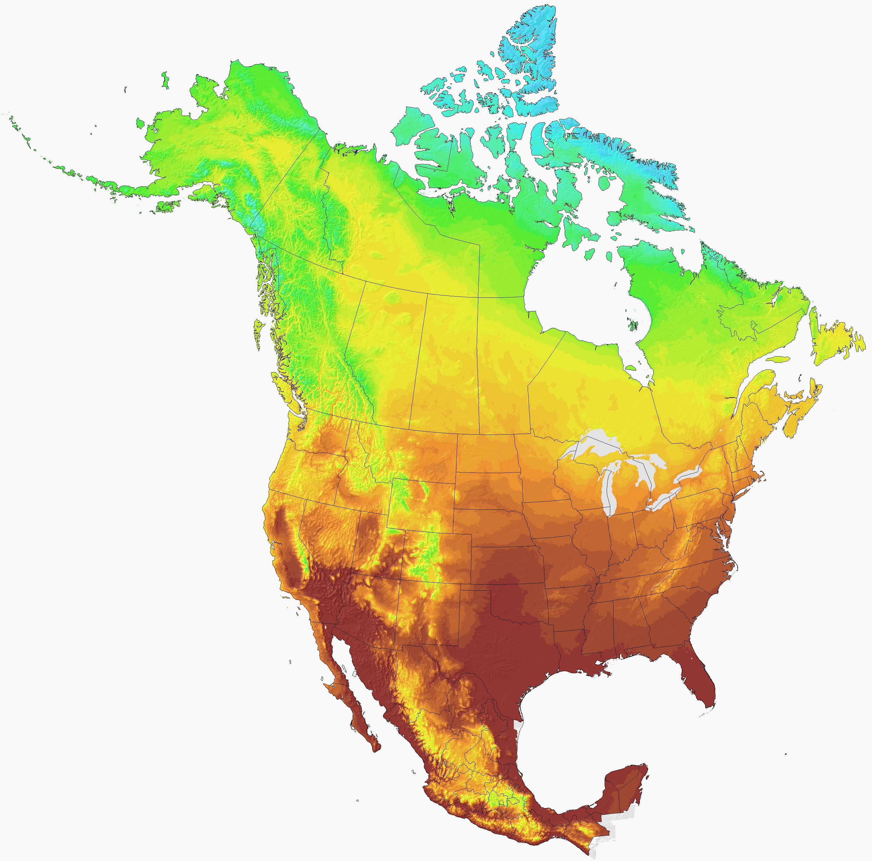
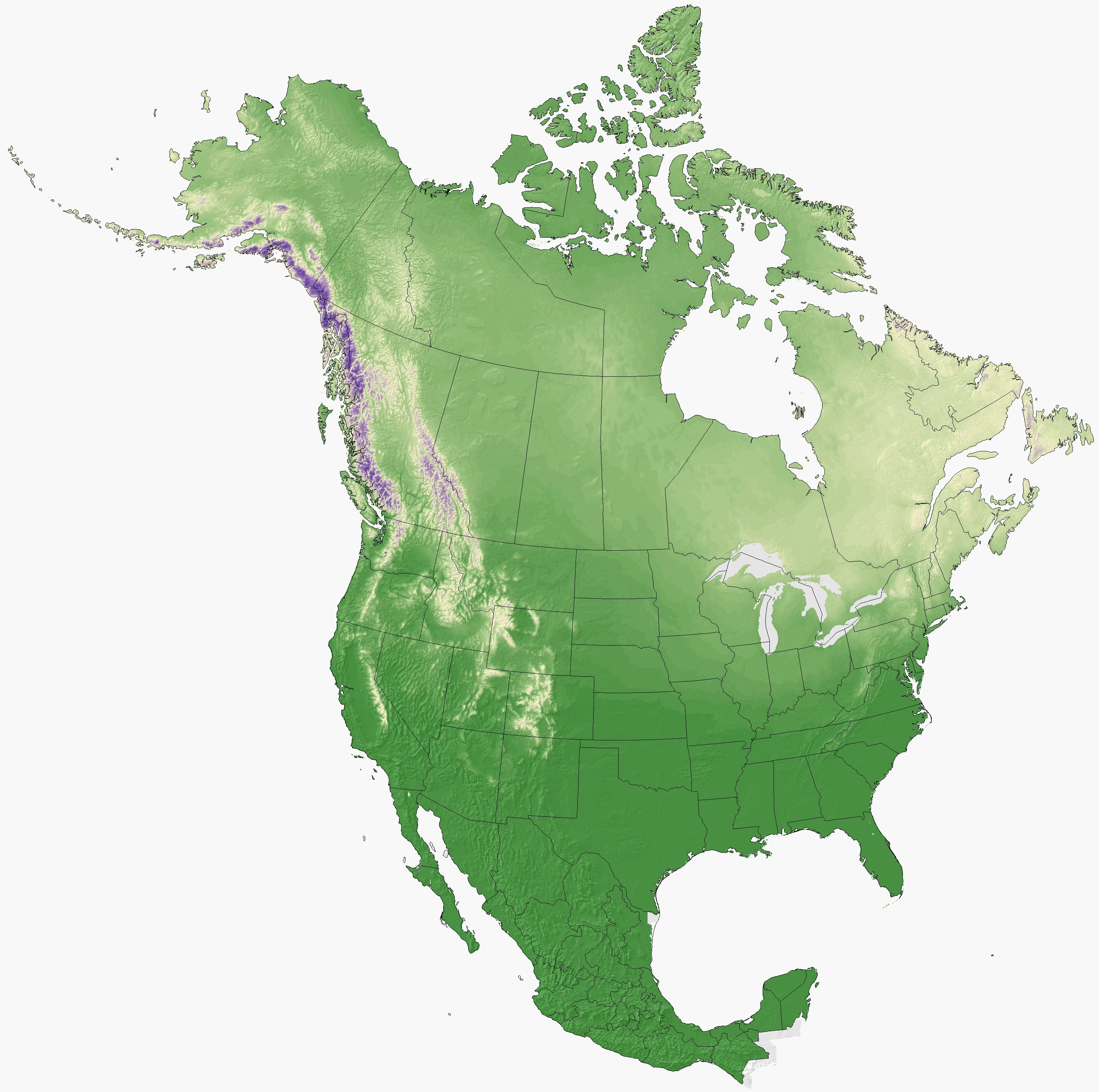
ClimateNA-ERA is an unpublished experimental version of the ClimateNA software that uses the monthly 0.1 degree ERA5-Land database [source] as a starting point for downscaling, using methodology described by Wang et al. (2016) and Namiiro et al (2025). The software package can generate historical (1950-2024) and future (CMIP6) climate grids and point estimates for 25 bioclimatic, 16 monthly and 16 seasonal variables.
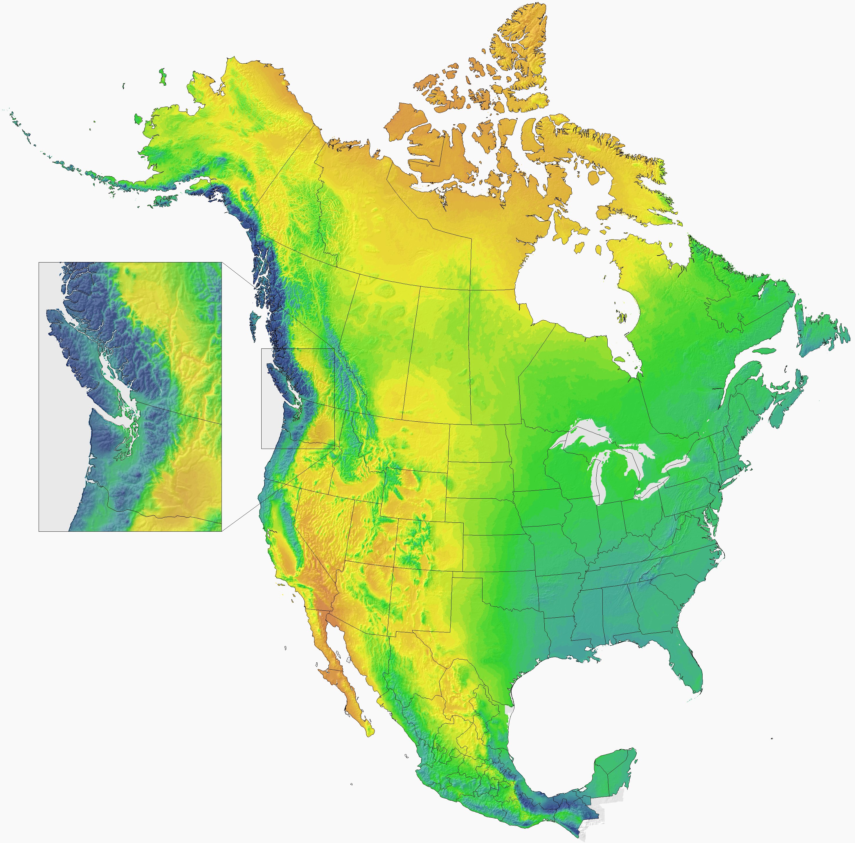
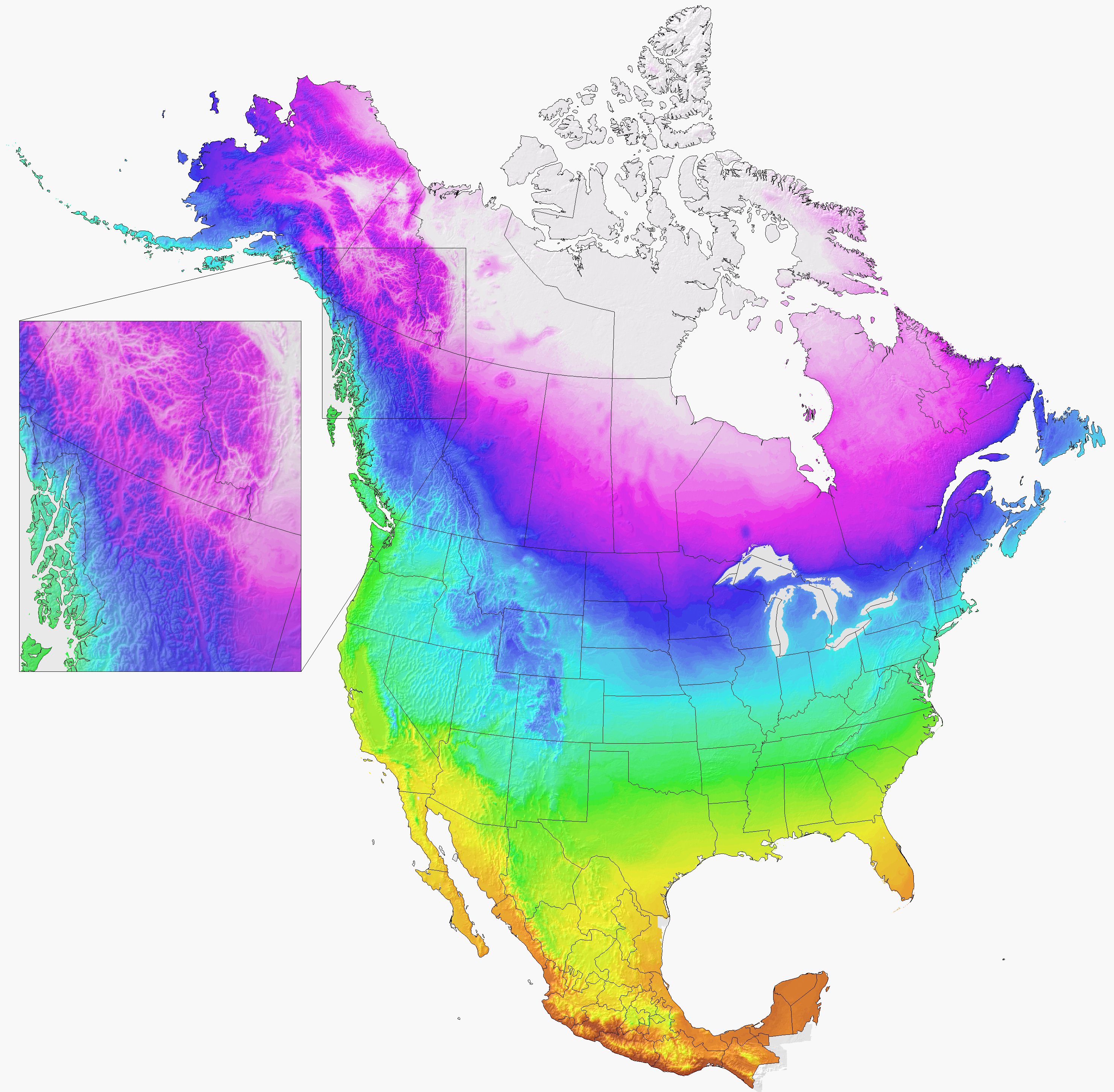
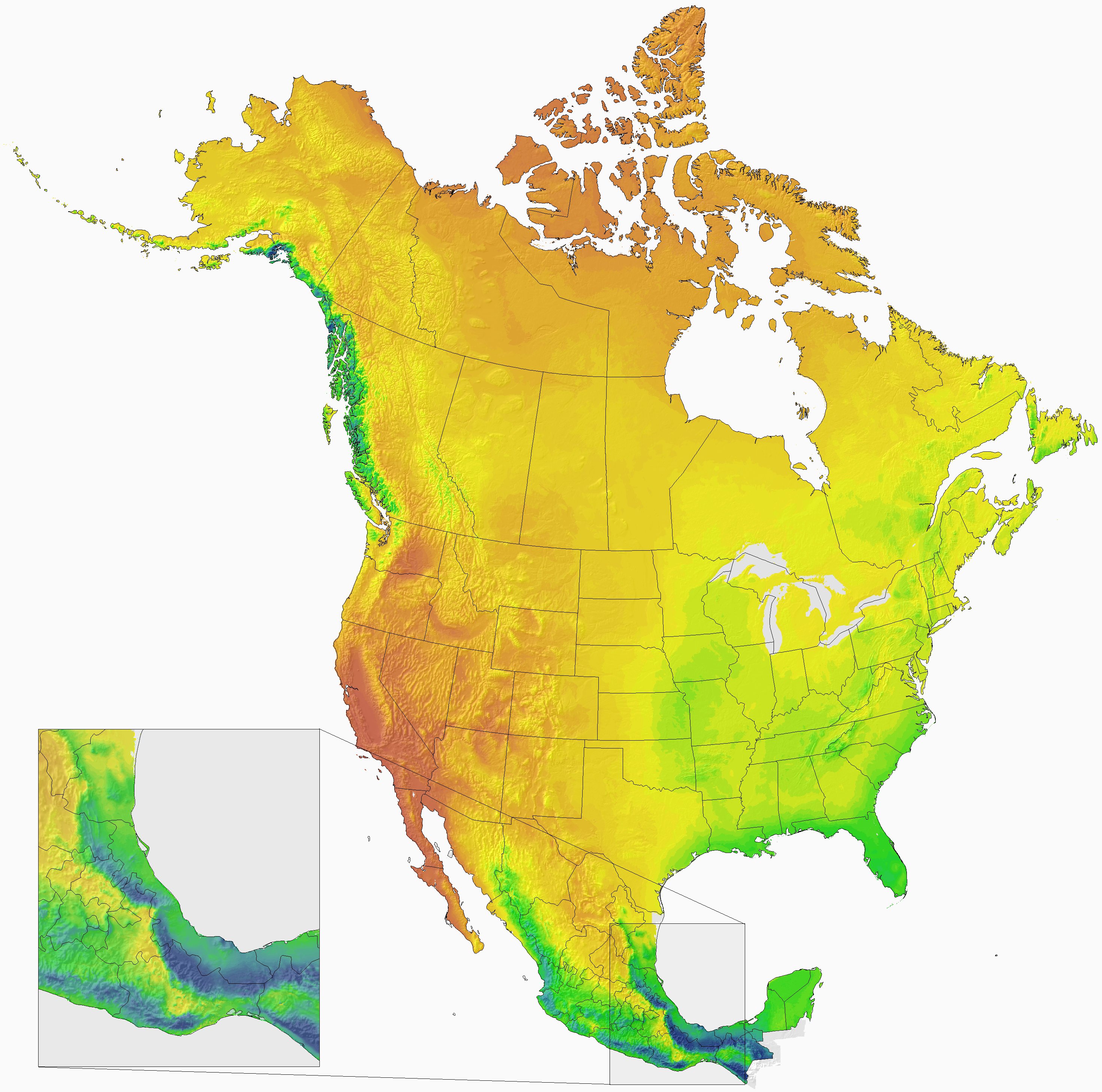
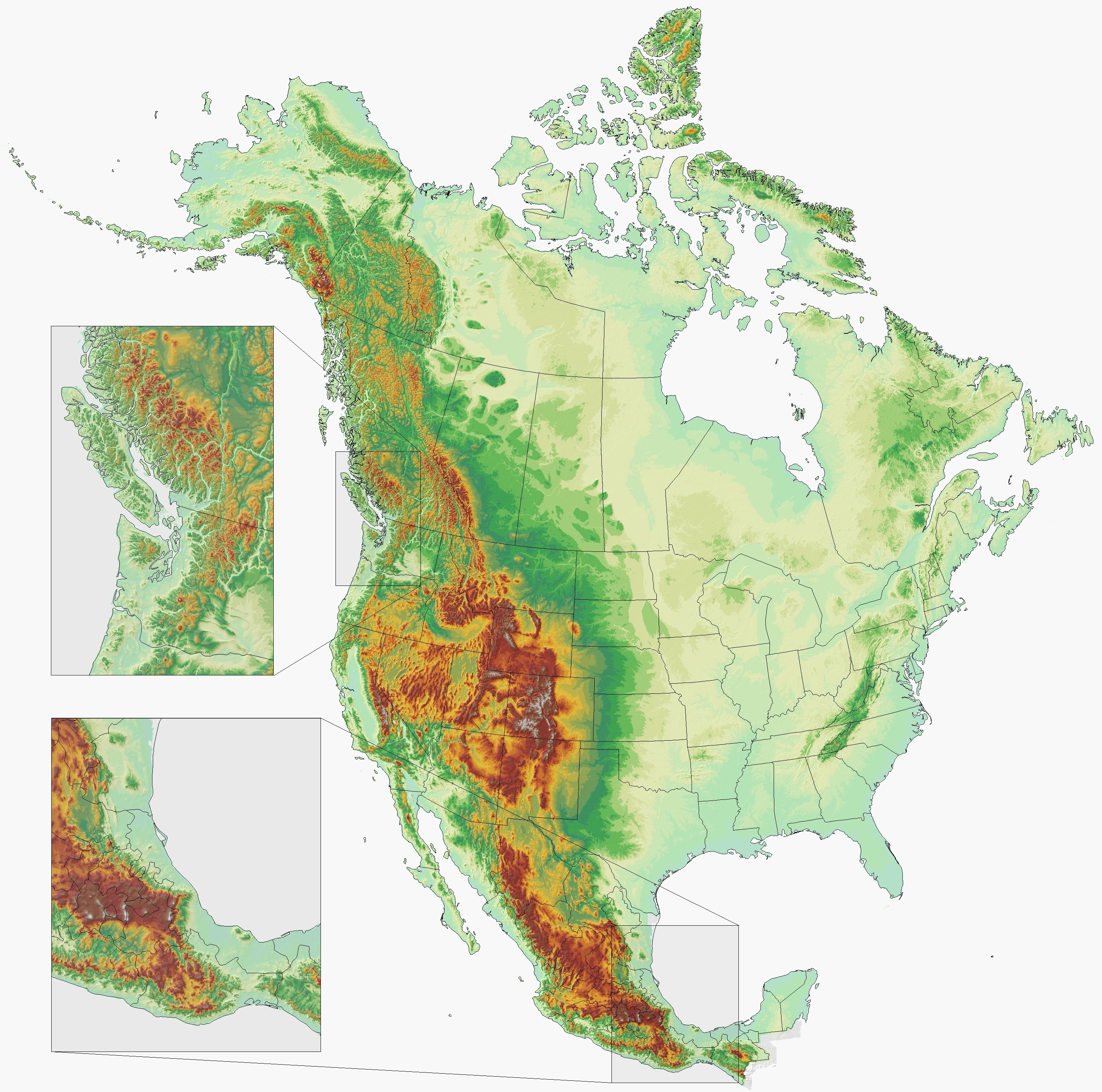
The climate grids were developed with a neural network that uses geographic and atmospheric information to model local weather patterns in complex terrain (e.g. see examples below, with the insets showing precipitation induced by orographic lift on the windward side, and rain shadows on the leeward side of major mountain ranges, as well as winter temperature inversions in northen valleys and basins.
Data downloads at 1 km resolution are available from the tables below, but you may also visually explore some sample grids: click on a thumbnails below and then zoom in or out of different areas (left-click mouse ![]() to zoom in/out), or view the RGB-GeoTIFFs in GIS (full resolution, without hillshade).
to zoom in/out), or view the RGB-GeoTIFFs in GIS (full resolution, without hillshade).
| Mean Annual Precipitation (View, GIS) | Mean Coldest Month Temp (View, GIS) | Mean Summer Precipitation (View, GIS) | Climate Moisture Deficit (View, GIS) |
 |
 |
 |
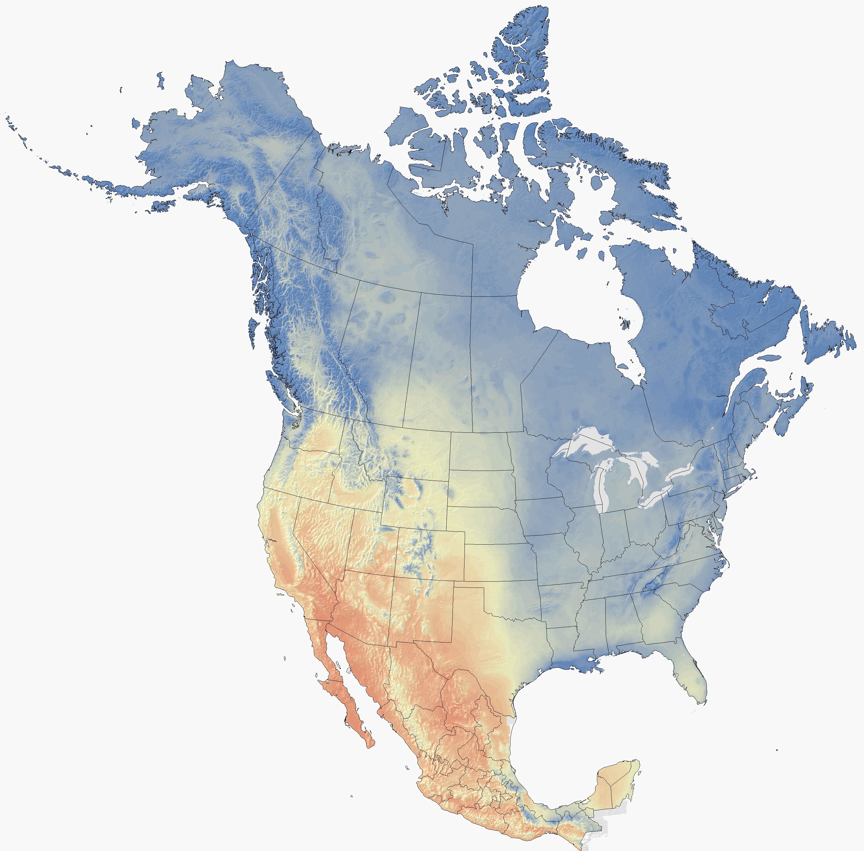 |
| Mean Annual Temperature (View, GIS) | Mean Warmest Month Temp (View, GIS) | Precipitation as Snow (View, GIS) | Reference Elevation Grid (View, GIS) |
 |
 |
 |
 |
ClimateNA-ERA software download and references
This program does not require installation. Download, unzip, and double click the executable file ClimateNA-ERA.exe. The program should run on all versions of Windows. If you receive the error message "COMCTL32.OCX missing", you have to install these libraryfiles. The program also runs on Linux, Unix and Mac systems with the free software Wine or MacPorts/Wine).

There is no peer reviewed article available yet, but in the meantime you can cite as follows: "Data was obtained using the software package ClimateNA-ERA, a variant of ClimateNA (Wang et al. 2016) that uses downscaling techniques described by Namiiro et al. (2025)."

Gridded data at 1 km resolution
This dataset was created with the ClimateNA-ERA v6.40 software package for historical and future 30-year normal periods. At present, only the 1961-1990 Normal period is available for testing and review:
Help file |
ClimateNA-ERA input file |
Reference elevation |
Area covered |
|---|---|---|---|
| Usage, variables: |
LAEA 1km input CSV: |
LAEA 1km geoTIFF: |
Shapefile: |
30 arcsec Historical 30-year climate normal periods |
|||
|---|---|---|---|
| 1940s (1931-1960) Bioclim: |
1950s (1941-1970) Bioclim: |
1960s (1951-1980) Bioclim: |
|
| 1970s (1961-1990) Bioclim: |
1980s (1971-2000) Bioclim: |
1990s (1981-2010) Bioclim: |
|
| 2000s (1991-2020) Bioclim: | (as a representation of current climate use the SSP2-2020s* projection below) | ||
Average ensemble scenarios1 |
27 Bioclimatic variables |
48 Monthly variables |
SSP1 (+2.6 W/m2) - Sustainability focus2 | 2020s3: |
2020s: |
|---|---|---|
| SSP2 (+4.5 W/m2) - Middle of the road | 2020s*: |
2020s*: |
| SSP3 (+7.0 W/m2) - Regional rivalry | 2020s: |
2020s: |
| SSP5 (+8.5 W/m2) - Fossil-fuel focus | 2020s: |
2020s: |
based on a variety of quality criteria and representativeness. For details on GCM selection, see Mahoney et al. (2022).
2) Average projected global warming by the 2080s for different Shared Socioeconomic Pathways (SSP) scenarios:
SSP1-2.6: 1.5-2.0°C; SSP2-4.5: 2.5-3.0°C; SSP3-7.0: 3.5-4.0°C; SSP5-5.8: 4.0-5.0°C.
3) Projections for 30-year normal periods: 2020s: 2011-2040, 2050s: 2041-2070, 2080s: 2071-2100.
*) SSP2-2020s is a good choice to represent current climate (midpoint of "middle of the road" climate normal estimate).
Scenario selection to quantify uncertainty for different regions of North America
If you want to quantify uncertainty in future projections, you need to work with a selection of multiple, individual models. This is easily done with the provided software for locations of interest (see video tutorial), and in addition we provide gridded data for nine high quality and representative AOGCMs.
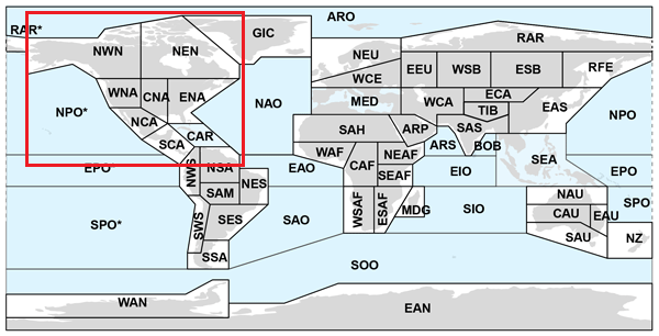
To help with the selection of a representative set of models for different regions of North America (or for the entire continent), we used the Katsavounidis-Kuo-Zhang (KKZ) algorithm, which selects an optimally representative set of future projections for different IPCC climate reference regions considering multiple climate variables (click on left panel dendrogram to visualize similarity among models):
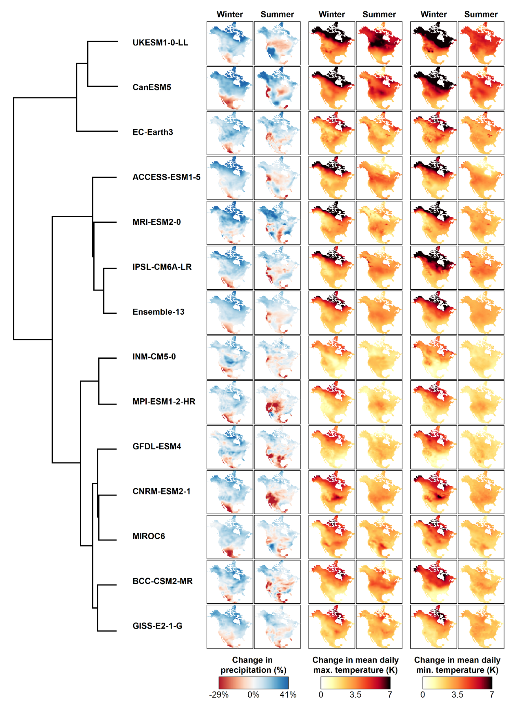
A common approach is to select a median, a pessimistic and an optimistic projection, i.e., a subset size of 3. For example, to assess uncertainty of future projections in the Northwest North America region (NWN) with a 3-model ensemble, you would choose the models: CNRM (median), EC (optimistic), and ACC (pessimistic) from the table below (compare with the dendrogram above). More models (rows 4 to 8) will provide increasingly better represenation of uncertainty in future predictions in multivariate space.
To include the sensitive "outlier" model UKES in the model selection process, use the lower portion of the table. If UKES is included, this scenario will almost always be picked second, as the most "pessimistic" model of global warming. UKES is not a very likely outcome, but if you work with a larger ensemble, you may include it as one possible outcome. For details on the GCM selection process, see Mahoney et al. (2022).
Subset size |
IPCC climate reference region1 |
North America |
||||||
|---|---|---|---|---|---|---|---|---|
NEN1 |
NWN |
WNA |
CNA |
ENA |
NCA |
SCA |
||
| Excluding UKESM1-0-LL | ||||||||
| 1 | CNRM2 | CNRM | MRI | MRI | GISS | MRI | GISS | CNRM |
| 2 | EC | EC | MPI | GFDL | ACC | GFDL | ACC | GFDL |
| 3 | GFDL | ACC | GISS | MIR | MRI | EC | MIR | EC |
| 4 | MRI | MPI | MIR | CNRM | GFDL | MIR | EC | GISS |
| 5 | ACC | GISS | EC | GISS | CNRM | CNRM | GFDL | MIR |
| 6 | GISS | MIR | CNRM | EC | EC | MPI | MPI | ACC |
| 7 | MPI | MRI | GFDL | MPI | MIR | ACC | MRI | MRI |
| 8 | MIR | GFDL | ACC | ACC | MPI | GISS | CNRM | MPI |
| Including UKESM1-0-LL | ||||||||
| 1 | CNRM | CNRM | MRI | ACC | EC | MRI | GISS | CNRM |
| 2 | UKES | UKES | UKES | UKES | UKES | UKES | UKES | UKES |
| 3 | EC | EC | MPI | CNRM | GFDL | GFDL | ACC | GFDL |
| 4 | MPI | MPI | GISS | GFDL | MRI | EC | MIR | EC |
| 5 | MRI | ACC | EC | MIR | MIR | MIR | EC | MRI |
| 6 | ACC | GISS | CNRM | EC | GISS | CNRM | GFDL | GISS |
| 7 | GISS | MRI | MIR | GISS | MPI | MPI | MPI | MIR |
| 8 | GFDL | MIR | GFDL | MPI | ACC | ACC | CNRM | ACC |
| 9 | MIR | GFDL | ACC | MRI | CNRM | GISS | MRI | MPI |
ENA, E.North-America; NCA, N.Central-America; SCA, S.Central-America.
2) Model abbreviations are: ACC, ACCESS-ESM1-5; CNRM, CNRM-ESM2-1; EC, EC-Earth3; GFDL, GFDL-ESM4; GISS, GISS-E2-1-G; MIR, MIROC6;
MPI, MPI-ESM1-2-HR; MRI, MRI-ESM2-0; and UKES, UKESM1-0-LL.