ClimateEU - Current, historical and projected climate data for Europe

Other climate data | Species range maps | Other data

ClimateEU: historical and projected climate data for Europe

On this page you can download the ClimateEU software and approximately 3,000 climate grids at 1 km resolution for historical climate (1901-2020) in monthly, annual, decadal, and 30-year steps and projected future climate (2020s, 2050s, 2080s) based on CMIP6 multi-model projections.

The database includes monthly base variables (Tmin, Tmax, Tave & Prec) as well as economically or biologically relevant (bioclim) variables such as growing and chilling degree days, beginning and end of frost free period, heating and cooling degree days, Hargrave's climate moisture deficit and reference evaporation, precipitation as snow, and seasonal variables.

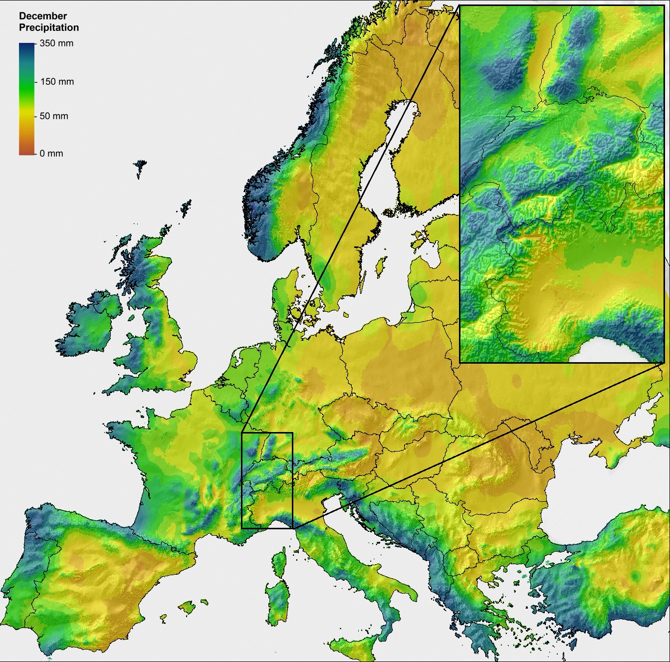
The climate grids were developed with a deep neural network that uses geographic and atmospheric information to model local weather patterns. Click on image on the right ( ) to see a higher resolution version, with the inset showing precipitation induced by orographic lift and rain shadows in the Alps region.

Subsequently, the ClimateEU software downscales the grids to higher resolutions with a digital elevation model in conjunction with local environmental lapse-rates. The software can also provide scale-free point estimates of climate variables for user-provided latitude, longitude and elevation coordinates.

Citation

A manuscript for a new deep-learning based ClimateEU software package including CMIP6 future projections [ClimateEU v5] is in preparation. In the meantime, you can cite our previous publication for use of the older CMIP5 dataset:

Marchi, M., Castellanos-Acuna, D., Hamann, A., Wang, T., Ray, D. Menzel, A. 2020. ClimateEU, scale-free climate normals, historical time series, and future projections for Europe. Scientific Data 7: 428. doi: 10.1038/s41597-020-00763-0

Video tutorials

Get started with these two video-tutorials. This first video explains the basic functionality of the software (1) interactive query of climate for locations, (2) processing spreadsheets of locations, (3) generating time series of climate, and (4) basic processing of gridded data. The second video explains in detail how to generate continental scale climate grids in projected coordinate systems, and how to automate generation of multiple climate surfaces for a variety of climate variables, historical time periods and future projections.

Tutorial 1: Learn the basic operation of the software

Tutorial 2: Learn how to mass-produce continental climate grids in a projection of your choice

Refererence files used on the tutorial above: 2.5km digital elevation model, outline of countries, and coastline mask in Albers projection.

Software download

This software can be used to query climate variables for any location, elevation and time period across Europe. The program does not require installation. Download, unzip, and double click the executable file ClimateEU.exe. The program should run on all versions of Windows. If you receive the error message "COMCTL32.OCX missing", you have to install these libraryfiles. The program also runs on Linux, Unix and Mac systems with the free software Wine or MacPorts/Wine).

ClimateEU v5.xx - covers Europe west of ~44 degree longitude and includes CMIP6 projections corresponding to IPCC Assessment Report 6 (2013) and ERA5-land historical data from 1950 to 2024. [currently under development - check back in February]

ClimateEU v4.63 - covers Europe west of ~44 degree longitude and includes CMIP5 projections corresponding to IPCC Assessment Report 5 (2013) and CRU-TS 4.05 historical data from 1901 to 2020.

Legacy CMIP3 multimodel future projections corresponding to IPCC Assessment Report 4 (2007). To use them, unzip the archive and place the .gcm files into the GCMdat folder of ClimateEU.

Gridded data at 5km resolution

[currently under development - check back in February] Meanwhile you can use our CMIP5 dataset available here.

Help file	ClimateEU input file	Elevation, ID reference	Area covered
Usage, variables, grid generator:	2.5 arcmin CSV:	2.5 arcmin geoTIFF:	Shapefile:

2.5 arcmin Historical 30-year climate normal periods
1931-1960 Bioclim: , Monthly:	1941-1970 Bioclim: , Monthly:	1951-1980 Bioclim: , Monthly:
1961-1990 Bioclim: , Monthly:	1971-2000 Bioclim: , Monthly:	1981-2010 Bioclim: , Monthly:
1991-2020 Bioclim: , Monthly:	(as a representation of current climate use the SSP2-2020s* projection below)

Average ensemble scenarios¹	27 Bioclimatic variables	48 Monthly variables
SSP1 (+2.6 W/m²) - Sustainability focus²	2020s³: , 2050s: , 2080s:	2020s: , 2050s: , 2080s:
SSP2 (+4.5 W/m²) - Middle of the road	2020s*: , 2050s: , 2080s:	2020s*: , 2050s: , 2080s:
SSP3 (+7.0 W/m²) - Regional rivalry	2020s: , 2050s: , 2080s:	2020s: , 2050s: , 2080s:
SSP5 (+8.5 W/m²) - Fossil-fuel focus	2020s: , 2050s: , 2080s:	2020s: , 2050s: , 2080s:

   ¹) The ensemble projections are averages across 8 CMIP6 models (ACC, CNRM, EC, GFDL, GISS, MIR, MPI and MRI) that were chosen
     based on a variety of quality criteria and representativeness. For details on GCM selection, see Mahoney et al. (2022).
   ²) Average projected global warming by the 2080s for different Shared Socioeconomic Pathways (SSP) scenarios:
       SSP1-2.6: 1.5-2.0°C; SSP2-4.5: 2.5-3.0°C; SSP3-7.0: 3.5-4.0°C; SSP5-5.8: 4.0-5.0°C.
   ³) Projections for 30-year normal periods: 2020s: 2011-2040, 2050s: 2041-2070, 2080s: 2071-2100.
   *) SSP2-2020s is a good choice to represent current climate (midpoint of "middle of the road" climate normal estimate).

Gridded data at 1km resolution

[currently under development - check back in February] Meanwhile you can use our CMIP5 dataset available here.

Help file	ClimateEU input file	Elevation, ID reference	Area covered
Usage, variables, grid generator:	30 arcsec CSV:	30 arcsec geoTIFF:	Shapefile:

30 arcsec Historical 30-year climate normal periods
1931-1960 Bioclim: , Monthly:	1941-1970 Bioclim: , Monthly:	1951-1980 Bioclim: , Monthly:
1961-1990 Bioclim: , Monthly:	1971-2000 Bioclim: , Monthly:	1981-2010 Bioclim: , Monthly:
1991-2020 Bioclim: , Monthly:	(as a representation of current climate use the SSP2-2020s* projection below)

Average ensemble scenarios¹	27 Bioclimatic variables	48 Monthly variables
SSP1 (+2.6 W/m²) - Sustainability focus²	2020s³: , 2050s: , 2080s:	2020s: , 2050s: , 2080s:
SSP2 (+4.5 W/m²) - Middle of the road	2020s*: , 2050s: , 2080s:	2020s*: , 2050s: , 2080s:
SSP3 (+7.0 W/m²) - Regional rivalry	2020s: , 2050s: , 2080s:	2020s: , 2050s: , 2080s:
SSP5 (+8.5 W/m²) - Fossil-fuel focus	2020s: , 2050s: , 2080s:	2020s: , 2050s: , 2080s:

Scenario selection to quantify uncertainty for different Counties and IPCC regions of Europe

[currently under development - check back in February] Meanwhile you can use our CMIP5 dataset available here.

If you want to quantify uncertainty in future projections, you need to work with a selection of multiple, individual models. This is easily done with the provided software for locations of interest (see video tutorial above), the pre-selected grids downloadable below, or it is also fairly straight-forward to generate custom grids with the help of some R code (included in the help file) if your data needs are different.

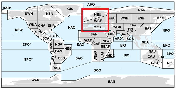
To help with the selection of a representative set of models for different regions of Africa (or for the entire continent), we used the Katsavounidis-Kuo-Zhang (KKZ) algorithm which selects an optimally representative set of future projections for different IPCC climate reference regions considering multiple climate variables:

IPCCregions

A common approach is to select a median, a pessimistic and an optimistic projection, i.e., a subset size of 3. For example, to assess uncertainty in the alps region, including Swtzerland and Austria (ch/at) with a 3-model ensemble, you would choose the models: GISS (median), MPI (optimistic), and EC (pessimistic) from the table below. Adding models (rows 4 to 8) will provide increasingly better representation of uncertainty in future predictions in multivariate space.

To include the sensitive "outlier" model UKES in the model selection process, use the lower portion of the table. If UKES is included, this scenario will almost always be picked second, as the most "pessimistic" model of global warming. UKES is not a very likely outcome, but if you work with a larger ensemble, you may include it as one possible outcome. For details on GCM selection process, see Mahoney et al. (2022)

Subset size	IPCC climate reference region (upper case) / groups of countries (lower case)											Europe
Subset size	NEU	WCE	MED	uk/ie	pt/es	fr/bl/lu	nl/dk/de	no/se/fi	ch/at	eu-ne	eu-se	Europe
Excluding UKESM1-0-LL
1	GISS	MRI	GFDL	MRI	CNRM	GISS	CNRM	GFDL	GISS	MRI	GFDL	GISS
2	EC	MPI	CNRM	ACC	EC	MIR	MPI	ACC	MPI	EC	CNRM	MPI
3	MRI	ACC	MPI	MIR	MPI	ACC	EC	MIR	EC	MPI	MIR	ACC
4	MPI	MIR	MIR	CNRM	GISS	GFDL	MRI	MPI	ACC	MIR	GISS	MIR
5	ACC	EC	GISS	GISS	MRI	MRI	ACC	EC	MIR	ACC	EC	MRI
6	CNRM	GFDL	EC	MPI	ACC	EC	GISS	MRI	CNRM	GFDL	MPI	EC
7	GFDL	CNRM	ACC	EC	MIR	MPI	MIR	CNRM	GFDL	CNRM	MRI	CNRM
8	MIR	GISS	MRI	GFDL	GFDL	CNRM	GFDL	GISS	MRI	GISS	ACC	GFDL
Including UKESM1-0-LL
1	CNRM	GISS	EC	CNRM	CNRM	GISS	CNRM	CNRM	CNRM	CNRM	EC	CNRM
2	UKES	UKES	UKES	UKES	UKES	UKES	UKES	UKES	MPI	UKES	UKES	UKES
3	EC	MPI	MPI	MPI	EC	MIR	MPI	MPI	UKES	EC	MIR	MPI
4	MPI	EC	MIR	MIR	MPI	ACC	EC	MIR	EC	MPI	CNRM	GFDL
5	MRI	MIR	CNRM	GISS	GISS	GFDL	MRI	EC	GFDL	GFDL	GISS	ACC
6	ACC	ACC	GISS	ACC	MRI	MRI	ACC	GISS	MIR	MIR	MRI	EC
7	GISS	GFDL	MRI	MRI	ACC	EC	GISS	MRI	GISS	ACC	GFDL	MIR
8	MIR	CNRM	ACC	EC	MIR	MPI	MIR	GFDL	ACC	MRI	MPI	GISS
9	GFDL	MRI	GFDL	GFDL	GFDL	CNRM	GFDL	ACC	MRI	GISS	ACC	MRI

   ¹) IPCC region abbreviations are: NEU, Northern Europe; WCE, West-Central Europe. Other groups: uk/ie/im, UK, Ireland; pt/es, Portugal, Spain;
       nl/dk/de, Netherlands, Denmark, Germany; no/sw/fi, Norway, Sweden, Finland; ch/at, Switzerland/Austria; ne-eu, northeastern European contries:
       Baltic to Romania; se-med, southeastern mediterannean countries:, Italy to Greece and Bulgaria;
   ²) Model abbreviations are: ACC, ACCESS-ESM1-5; CNRM, CNRM-ESM2-1; EC, EC-Earth3; GFDL, GFDL-ESM4; GISS, GISS-E2-1-G; MIR, MIROC6;
       MPI, MPI-ESM1-2-HR; MRI, MRI-ESM2-0; and UKES, UKESM1-0-LL.

Below, you can find a table with individual scenario downloads for uncertainty analysis. This is not the full set of SSPs is not typically necessary for a meaningful uncertainty analysis. The selection below will be suitable to quantify medium term (2050s) and long term (2080s) uncertainty in projections, as well as the dependence of outcomes on two SSPs.

Individual GCM downloads for uncertainty analysis

[currently under development - check back in February] Meanwhile you can use our CMIP5 dataset available here.

AOGCM	SSP2 (+4.5 W/m²) - Middle of the road		SSP5 (+8.5 W/m²) - Fossil-fuel focus
AOGCM	27 Bioclimate variables	48 Monthly variables	27 Bioclimate variables	48 Monthly variables
ACCESS-ESM1-5 (ACC)	2050s: , 2080s:	2050s: , 2080s:	2050s: , 2080s:	2050s: , 2080s:
CNRM-ESM2-1 (CNRM)	2050s: , 2080s:	2050s: , 2080s:	2050s: , 2080s:	2050s: , 2080s:
EC-Earth3 (EC)	2050s: , 2080s:	2050s: , 2080s:	2050s: , 2080s:	2050s: , 2080s:
GFDL-ESM4 (GFDL)	2050s: , 2080s:	2050s: , 2080s:	2050s: , 2080s:	2050s: , 2080s:
GISS-E2-1-G (GISS)	2050s: , 2080s:	2050s: , 2080s:	2050s: , 2080s:	2050s: , 2080s:
MIROC6 (MIR)	2050s: , 2080s:	2050s: , 2080s:	2050s: , 2080s:	2050s: , 2080s:
MPI-ESM1-2-HR (MPI)	2050s: , 2080s:	2050s: , 2080s:	2050s: , 2080s:	2050s: , 2080s:
MRI-ESM2-0 (MRI)	2050s: , 2080s:	2050s: , 2080s:	2050s: , 2080s:	2050s: , 2080s:
UKESM1-0-LL (UKES)	2050s: , 2080s:	2050s: , 2080s:	2050s: , 2080s:	2050s: , 2080s:

Acknowledgements

This research has, in part, been sponsored by the Alexander von Humboldt foundation and an NSERC Discovery Grant.