The relativistic propagator,
![]() is defined to
satisfy a Green's function equation
is defined to
satisfy a Green's function equation
| (6.64) |
The propagator is a ![]() matrix corresponding to the
dimensionality of
matrix corresponding to the
dimensionality of ![]() matrices.
Note that the definition of the relativistic propagator differs from the
nonrelativistic counterpart: the differential operator
matrices.
Note that the definition of the relativistic propagator differs from the
nonrelativistic counterpart: the differential operator
![]() occurring in
the nonrelativistic equation has been multiplied by
occurring in
the nonrelativistic equation has been multiplied by ![]() in the
relativistic equation in order to form the covariant operator
in the
relativistic equation in order to form the covariant operator
![]() .
.
Suppressing the indices we have
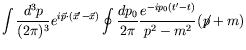
We can compute the free-particle propagator,
![]() , using
, using
| (6.66) |
by Fourier transforming to momentum space.
![]() depends only on the interval
depends only on the interval ![]() .
This property is a manifestation of the homogeneity of space and time,
and is general would not be valid for the interacting propagator
.
This property is a manifestation of the homogeneity of space and time,
and is general would not be valid for the interacting propagator
![]() .
We have
.
We have
| (6.67) |
This gives
| (6.68) |
Solving for the Fourier amplitude ![]() and reverting to the matrix
shorthand, we find
and reverting to the matrix
shorthand, we find
| (6.69) |
A prescription for how to handle the singularity at ![]() or
(
or
(
![]() ) is needed.
This comes from the boundary conditions put on
) is needed.
This comes from the boundary conditions put on
![]() in
the integration.
in
the integration.
The interpretation given to the Green's function
![]() is
that it represents the wave produced at the point
is
that it represents the wave produced at the point ![]() by a unit
source located at the point
by a unit
source located at the point ![]() .
The Fourier components of such a localized point source contain many
momenta larger than
.
The Fourier components of such a localized point source contain many
momenta larger than ![]() , the reciprocal of the electron Compton
wavelength, and we expect that positrons as well as electrons may be
created at
, the reciprocal of the electron Compton
wavelength, and we expect that positrons as well as electrons may be
created at ![]() by the source.
However, a necessary physical requirement of the hole theory is that
the wave propagating from
by the source.
However, a necessary physical requirement of the hole theory is that
the wave propagating from ![]() into the future consist only of
positive-energy electron and positron components.
Since positive-energy positrons and electrons are represented by wave
functions with positive frequency time behaviour
into the future consist only of
positive-energy electron and positron components.
Since positive-energy positrons and electrons are represented by wave
functions with positive frequency time behaviour
![]() can
contain in the future
can
contain in the future
![]() , only positive-frequency
components.
, only positive-frequency
components.
We perform the ![]() integration along the contour in the complex
integration along the contour in the complex
![]() -plane.
For
-plane.
For ![]() , the contour is closed in the lower half-plane and
includes the positive-frequency pole at
, the contour is closed in the lower half-plane and
includes the positive-frequency pole at
![]() only.
This gives
only.
This gives
 |
|||
| (6.70) |
so that the wave at
![]() contains
positive-frequency components only.
For
contains
positive-frequency components only.
For ![]() , the contour can be closed above, including the pole
at
, the contour can be closed above, including the pole
at
![]() .
This gives
.
This gives
| (6.71) |
showing the propagator to consist of negative-frequency waves for
![]() .
Any other choice of contour leads to negative-energy waves propagating
into the future or positive-energy waves propagating into the past.
Moreover, the negative-energy waves propagating into the past that we
have just found are welcome; they are the positive-energy positrons.
The origin of the negative-energy waves is the pole at
.
Any other choice of contour leads to negative-energy waves propagating
into the future or positive-energy waves propagating into the past.
Moreover, the negative-energy waves propagating into the past that we
have just found are welcome; they are the positive-energy positrons.
The origin of the negative-energy waves is the pole at
![]() , which was not present in the
nonrelativistic theory.
, which was not present in the
nonrelativistic theory.
The choice of the contour is summarised by adding a small positive
imaginary part to the denominator, or simply taking
![]() , where the limit
, where the limit
![]() is
understood:
is
understood:
| (6.72) |
The two integrations can be combined by introducing projection
operators and changing ![]() to
to ![]() in the
negative-frequency part:
in the
negative-frequency part:
| (6.73) |
with ![]() .
.
Equivalently, writing for normalized plane-wave solutions, we find
| (6.74) |
We see that
![]() carries the positive-energy solutions
carries the positive-energy solutions
![]() forward in time and the negative-energy ones
forward in time and the negative-energy ones ![]() backward in time
backward in time
The minus sign in the second equation results from the difference of the direction of propagation in time between (6.75) and (6.76).
![]() is known as the Feynman propagator.
This spin-1/2 propagator is related to the Klein-Gordon propogator by
is known as the Feynman propagator.
This spin-1/2 propagator is related to the Klein-Gordon propogator by
| (6.77) |
From the free propagator
![]() we may formally construct
the complete Green's function and the
we may formally construct
the complete Green's function and the ![]() -matrix elements, that is,
the amplitudes for various scattering processes of electrons and
positrons in the presence of force fields.
The exact Feynman propagator
-matrix elements, that is,
the amplitudes for various scattering processes of electrons and
positrons in the presence of force fields.
The exact Feynman propagator
![]() satisfies
(6.65) and can be expressed in terms of a superposition of
free Feynman propagators
satisfies
(6.65) and can be expressed in terms of a superposition of
free Feynman propagators
This is the relativistic counterpart of the Lippmann-Schwinger
equation.
Another notation for
![]() is
is
![]() .
This integral equation determines the complete propagator
.
This integral equation determines the complete propagator
![]() in terms of the free-particle propagator
in terms of the free-particle propagator
![]() .
.
Proceeding in analogy to the nonrelativistic treatment, the iteration of the integral equation yields the following multiple scattering expansion
| (6.80) | |||
Equation 6.78 can be viewed as an inhomogeneous Dirac equation
of the form
![]() which is solved by the
Green's function techniques as follows
which is solved by the
Green's function techniques as follows
| (6.81) |
The exact solution of the Dirac equation with the Feynman boundary conditions, is
where ![]() is the free-particle solution.
The scattering wave contains only positive frequencies in the future
and negative frequencies in the past
is the free-particle solution.
The scattering wave contains only positive frequencies in the future
and negative frequencies in the past
![$\displaystyle \int d^3p \sum_{r=1}^2 \psi_P^r(x)
[-ie \int d^4y \overline{\psi}_P^r(y) \not{\!\!A}(y) \Psi(y) ]
\quad\textrm{as}\quad t \rightarrow +\infty ,$](img2871.png) |
(6.83) | ||
![$\displaystyle \int d^3p \sum_{r=3}^4 \psi_P^r(x)
[+ie \int d^4y \overline{\psi}_P^r(y) \not{\!\!A}(y) \Psi(y) ]
\quad\textrm{as}\quad t \rightarrow -\infty .$](img2874.png) |
(6.84) |