We seek a relativistic covariant equation of the form
which is first order in the time derivative and will have positive definite probability density. Assuming such an equation is also linear in the space derivatives, we can write
| (5.2) |
Using operator notation we have
For invariance under spatial rotation, the ![]() can not be numbers
and
can not be numbers
and ![]() can not be a scalar.
In analogy with the spin wave function of nonrelativistic quantum
mechanics, we choose
can not be a scalar.
In analogy with the spin wave function of nonrelativistic quantum
mechanics, we choose ![]() to be a vector, and
to be a vector, and ![]() and
and ![]() to be matrices.
Explicitly,
to be matrices.
Explicitly,
| (5.4) |
We thus have ![]() coupled first-order equations.
coupled first-order equations.
These equations must
For the first condition to be satisfied, each component of ![]() must satisfy the Klein-Gordon equation.
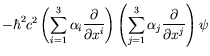
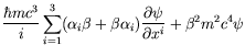
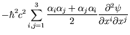
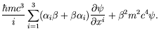
Applying the operator (5.1) twice gives
must satisfy the Klein-Gordon equation.
Applying the operator (5.1) twice gives
 |
|||
 |
|||
 |
|||
 |
(5.5) |
To obtain the Klein-Gordon equation the following must be satisfied
where ![]() represents an
represents an ![]() unit matrix.
We will not write the unit matrix explicitely in the wave equation
unless it is required for clarity.
This should not create any confusion since matrices can only equal
matrices.
unit matrix.
We will not write the unit matrix explicitely in the wave equation
unless it is required for clarity.
This should not create any confusion since matrices can only equal
matrices.
No terms in the Hamiltonian can have any space or time coordinates.
Such terms would have the property of space-time dependent energies
and would give rise to forces.
Space and time derivatives can only appear in ![]() and
and ![]() ,
but not in
,
but not in ![]() and
and ![]() , since the equation is to be linear
in these derivatives.
Thus
, since the equation is to be linear
in these derivatives.
Thus ![]() and
and ![]() are independent of
are independent of
![]() and hence commute with them.
and hence commute with them.
Since the Hamiltonian must be hermitian, ![]() and
and ![]() must
be hermitian matrices.
Since the matrices are hermitian they must be square.
must
be hermitian matrices.
Since the matrices are hermitian they must be square.
Since ![]() and
and ![]() anticommute according to
equation 5.7, they are traceless.
This can be seen as follows:
anticommute according to
equation 5.7, they are traceless.
This can be seen as follows:
| (5.9) |
where the last line follows from the cyclic property of the trace.
The choice of ![]() and
and ![]() is not unique.
All matrices related to these by any unitary
is not unique.
All matrices related to these by any unitary ![]() matrix
matrix ![]() (which preserves the anti-commutation relations) are allowed:
(which preserves the anti-commutation relations) are allowed:
![]() and
and
![]() .
.
Since
![]() , the eigenvalues of
, the eigenvalues of ![]() and
and ![]() are
are ![]() .
Since the trace is the sum of eigenvalues
.
Since the trace is the sum of eigenvalues ![]() and
and ![]() , must
be of even dimensions.
For
, must
be of even dimensions.
For ![]() , only three anti-commuting matrices exist (the Pauli
matrices).
Thus the smallest dimension allowed is
, only three anti-commuting matrices exist (the Pauli
matrices).
Thus the smallest dimension allowed is ![]() .
.
If one matrix is diagonal, the others can not be diagonal or they would
commute with the diagonal matrix.
We can write a representation that is hermitian, traceless, and has
eigenvalues of ![]() :
:
where ![]() are the
are the ![]() Pauli matrices and
Pauli matrices and ![]() is the
is the
![]() unit matrix.
unit matrix.