We treat the proton as a structureless Dirac particle.
If we know the current of the proton, ![]() , we can calculate
using Maxwell's equations the field it generates.
We first find the electromagnetic field produced by the proton.
The potential satisfies
, we can calculate
using Maxwell's equations the field it generates.
We first find the electromagnetic field produced by the proton.
The potential satisfies
| (7.133) |
where we are working in the Lorentz gauge.
We are free to choose the most conveniant gauge.
We are working in the Heaviside-Lorentz system of units.
In the Gaussian system of units a ![]() would appear in front of the
current.
To solve the equation, we introduce the Green function,
would appear in front of the
current.
To solve the equation, we introduce the Green function, ![]() ,
define by
,
define by
| (7.134) |
Its Fourier representation is
| (7.135) |
where
![]() , for
, for ![]() .
.
In analogy with the Dirac propagator, we append an infinitesimally
small positive imaginary part to ![]() .
This is equivalent to adding a small negative imaginary mass
.
This is equivalent to adding a small negative imaginary mass
| (7.136) |
This is the so-called ``photon propagator''.
The interacting photon is said to be ``virtual'', or
``off-mass-shell'', and ![]() is termed the mass squared of the
virtual photon.
That the photons are virtual is clear since for real photons, the
energy-momentum vector
is termed the mass squared of the
virtual photon.
That the photons are virtual is clear since for real photons, the
energy-momentum vector ![]() satisfies
satisfies ![]() , whence the
propagator becomes infinite.
Likewise for the Dirac equation, the propagator becomes infinite when
the quanta are on their ``mass shell'';
, whence the
propagator becomes infinite.
Likewise for the Dirac equation, the propagator becomes infinite when
the quanta are on their ``mass shell''; ![]() .
.
The Feynman propagator for electromagnetic radiation is
| (7.137) |
Using Green's function techniques, the solution for the potential is
| (7.138) |
since
| (7.139) |
In a more general gauge
| (7.140) |
It carries Lorentz indices because the photon is a spin-1 particle.
In our case, the tensor ![]() is just proportional to
is just proportional to
![]() so that the tensor indices can be discarded for
convenience by defining
so that the tensor indices can be discarded for
convenience by defining
![]() .
.
We could also, of course, append a solution of the homogeneous
equation here.
However, the solution which we wish for ![]() is that which
vanishes in the absence of a transition density
is that which
vanishes in the absence of a transition density ![]() (this is
true for all our Green function equations).
(this is
true for all our Green function equations).
The ![]() -matrix is
-matrix is
| (7.141) |
![]() is the current of the
electron.
The problem now is to decide what to choose for the proton current
is the current of the
electron.
The problem now is to decide what to choose for the proton current
![]() ?
Its reasonable to try
?
Its reasonable to try
| (7.142) |
where ![]() is the proton charge.
is the proton charge.
![]() and
and
![]() represent the initial and
final plane wave solutions for a free proton.
Using plane-wave solutions for a proton gives
represent the initial and
final plane wave solutions for a free proton.
Using plane-wave solutions for a proton gives
| (7.143) |
where ![]() and
and ![]() are the initial and final proton four-momentum
and
are the initial and final proton four-momentum
and ![]() is its mass.
is its mass.
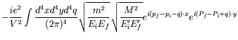
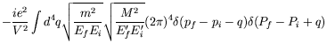
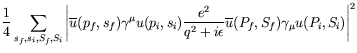
We now get for the ![]() -matrix
-matrix
![$\displaystyle \cdot \int \frac{d^4q}{(2\pi)^4}
e^{-iq\cdot(x-y)} \left( \frac{-...
...e V}}
e^{i(P_f-P_i)\cdot y} \overline{u}(P_f,S_f) \gamma^\mu u(P_i,S_i) \right]$](img3654.png) |
|||
 |
|||
 |
|||
 |
|||
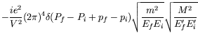
| (7.144) |
Notice the symmetry in electron and proton variables.
This gives the electron-proton scattering amplitude to lowest order in
![]() .
Higher order interaction effects which distort the plane waves that
were inserted in the currents have been ignored.
The expression for the
.
Higher order interaction effects which distort the plane waves that
were inserted in the currents have been ignored.
The expression for the ![]() -matrix may be represented by a Feynman
diagram as shown in figure 7.4.
-matrix may be represented by a Feynman
diagram as shown in figure 7.4.
For each line and intersection of the graph there corresponds a unique
factor in the ![]() -matrix.
In addition,
-matrix.
In addition, ![]() always contains a four-dimensional
always contains a four-dimensional
![]() -function expressing overall energy-momentum conservation.
A solid line with an arrow pointing toward positive time represents
the electron and a double line the proton.
The wavy line represents the influence of the electromagnetic
interaction, which is expressed in the matrix element by the
reciprocal of the square of the momentum transfer, or the inverse
d'Alembertian in momentum space.
We refer to this line as representing a ``virtual photon'' exchanging
four-momentum
-function expressing overall energy-momentum conservation.
A solid line with an arrow pointing toward positive time represents
the electron and a double line the proton.
The wavy line represents the influence of the electromagnetic
interaction, which is expressed in the matrix element by the
reciprocal of the square of the momentum transfer, or the inverse
d'Alembertian in momentum space.
We refer to this line as representing a ``virtual photon'' exchanging
four-momentum
![]() between the electron and proton.
The amplitude for the virtual photon to propagate between the two
currents is
between the electron and proton.
The amplitude for the virtual photon to propagate between the two
currents is
![]() .
At the points (or vertices) on which the photon lands there operate
factors
.
At the points (or vertices) on which the photon lands there operate
factors ![]() sandwiched between spinors
sandwiched between spinors
![]() representing the free, real incident and outgoing particles.
To get the spinor factor in expressions such as these, the rule is to
start at the ingoing fermion line
representing the free, real incident and outgoing particles.
To get the spinor factor in expressions such as these, the rule is to
start at the ingoing fermion line ![]() and follow the line through until
the end, inserting vertices and propagators in the right order, until
you reach the outgoing state
and follow the line through until
the end, inserting vertices and propagators in the right order, until
you reach the outgoing state ![]() .
There is a uniform rule for the factors of
.
There is a uniform rule for the factors of ![]() :
: ![]() for each vertex
and
for each vertex
and ![]() for each internal line in the graph.
for each internal line in the graph.
We now form a transition rate per unit volume by dividing ![]() by the time interval of observation
by the time interval of observation ![]() and by the spatial volume
and by the spatial volume ![]() of the interaction region.
This gives
of the interaction region.
This gives
| (7.145) |
where
| (7.146) |
is a Lorentz invariant matrix element and will be called the invariant
amplitude.
The choice of this name is quite natural since the matrix element
consits of scalar products of four-vectors, which is Lorentz
invariant.
We have used, in analogy to before, the square of the
![]() -function
-function
| (7.147) |
where the four-dimensional delta-function is just the product of four one-dimensional delta-functions.
We divide the transition rate per unit volume by the flux of incident
particles
![]() and by the number of target particles per
unit volume, which is just
and by the number of target particles per
unit volume, which is just ![]() .
Since the normalization of the wave function was performed in such a
way that there is just one particle in the normalized volume
.
Since the normalization of the wave function was performed in such a
way that there is just one particle in the normalized volume ![]() .
To get a physical cross-section, we must sum over a given group of
final states of the electron and proton corresponding to the
laboratory conditions for observing the process.
The number of final states of a specified spin in the momentum
interval
.
To get a physical cross-section, we must sum over a given group of
final states of the electron and proton corresponding to the
laboratory conditions for observing the process.
The number of final states of a specified spin in the momentum
interval ![]() is
is
| (7.148) |
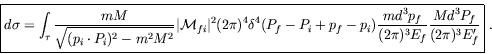
and thus the six-fold differential cross-section for transitions to the
final states in the interval ![]() is
is
| (7.149) |
The physics lies in
![]() , the square of the invariant
amplitude.
There is a factor
, the square of the invariant
amplitude.
There is a factor ![]() for each external fermion line, that is, for
each Dirac particle incident upon or emerging from the interaction.
The phase-space factor for each final particle is
for each external fermion line, that is, for
each Dirac particle incident upon or emerging from the interaction.
The phase-space factor for each final particle is
![]() .
Each final particle gives rise to the factor
.
Each final particle gives rise to the factor
![]() .
The following combination forms a Lorentz invariant volume element in
momentum space as can be seen from
.
The following combination forms a Lorentz invariant volume element in
momentum space as can be seen from
| (7.150) |
which is invariant provided ![]() is time-like, as is the case here.
is time-like, as is the case here.
In the factor
![]() ,
,
![]() is the flux and for
collinear beams, which is the number of particles per unit area which
run by each other per unit time,
is the flux and for
collinear beams, which is the number of particles per unit area which
run by each other per unit time,
| (7.151) |
which is the particle density times the relative velocity.
We have required that the velocity vectors are collinear.
When
![]() is combined with the normalization factor for two
incident particles, it forms a Lorentz invariant expression
is combined with the normalization factor for two
incident particles, it forms a Lorentz invariant expression
| (7.152) |
The last expression can be seen by
| (7.153) |
Consequently the naive flux factor in the cross-section has in general to be replaced by the Lorentz-invariant flux factor. In the case of collinear collisions, both results are idential. This shows that the total cross-section is invariant under Lorentz transformations along the direction of motion of the incident beams. We can write the invariant form
 |
(7.154) |
The two-particle Lorentz-invariant phase space is
| (7.155) |
where ![]() is the
is the ![]() Mandelstram variable.
Mandelstram variable.
Averaging over initial and summing over final spins
 |
|||
| (7.156) |
Note that squaring the amplitude which contained the scalar product of two Lorentz scalars has lead to the contraction of two tensors, i.e. a double sum. One often abbriviates this as
| (7.157) |
were ![]() is the lepton (i.e. electron) tensor and
is the lepton (i.e. electron) tensor and
![]() the hardonic (i.e. proton) tensor:
the hardonic (i.e. proton) tensor:
| (7.158) |
and similarily
| (7.159) |
The factorization remains meaningful as long as a single virtual photon is exchanged in the scattering process, even if the transition currents become more complicated than those here.
Returning to evaluating the traces, the first trace is
| (7.160) |
The second trace is of the same form
| (7.161) |
The square of the invariant amplitude now becomes
| (7.162) |
To evaluate the scattering cross-section any further, the frame of
reference has to be specified.
Usually calculations take their simplist form in the center-of-mass
system.
However, electron-proton scatter experiments are mostly performed
using a fixed target in the laroratory frame (except HERA).
Therefore we evaluate ![]() in the laboratory frame in which the
initial proton is at rest:
in the laboratory frame in which the
initial proton is at rest:
| (7.163) | |||
| (7.164) | |||
| (7.165) |
We also write
| (7.166) |
and use
| (7.167) |
to get
| (7.168) |
Using
![]() , we
calculate
, we
calculate
| (7.169) |
and require
| (7.170) |
We obtain
| (7.171) |
For electrons of energy much less than the proton rest mass, we resurrect the earlier result of scattering in a static Coulomb field,
| (7.172) |
where
| (7.173) |
which is the Mott cross-section.
When the proton recoil becomes important, the electron may be treated as extremely relativistic and the electron rest mass is negligible with respect to the electron energy
| (7.174) |
To evaluate the matrix element we re-express ![]() in terms of the
electron recoil using energy-momentum conservation
in terms of the
electron recoil using energy-momentum conservation
![]() and
and
| (7.175) |
Using
![]() , we have
, we have
| (7.176) |
In the limit
![]() , conservation of energy gives
, conservation of energy gives
| (7.177) |
Thus
| (7.178) |
The ![]() -dependent second term is found to originate from the fact
that the target is a spin-1/2 particle.
This term is absence when the collision of electrons with spin-0
particles is calculated.
-dependent second term is found to originate from the fact
that the target is a spin-1/2 particle.
This term is absence when the collision of electrons with spin-0
particles is calculated.
The differential cross-section thus becomes
| (7.179) |
This derivation has treated the proton as a heavy electron of mass
![]() .
The description is incomplete since it fails to take into account the
proton structure and anomalous magnetic moment.
A complete description of the proton leads to modifications which are
important at large energies exceeding several hundred MeV, since the de
Broglie wavelength of the electron is so small that the substructure of
the proton becomes detectable.
.
The description is incomplete since it fails to take into account the
proton structure and anomalous magnetic moment.
A complete description of the proton leads to modifications which are
important at large energies exceeding several hundred MeV, since the de
Broglie wavelength of the electron is so small that the substructure of
the proton becomes detectable.
In a complete treatment for very high energies (several 100 MeV), the formula has to be modified by introducing electric and magnetic form factors representing the internal structure of the proton. This yields the so-called Rosenbluth formula.
Our result would apply with great accuracy, however, to the scattering of electrons and muons which both are structureless Dirac particles.
![\begin{figure}\begin{center}
\begin{picture}(280,125)(-30,-10)
\SetWidth{0.75}
%...
...5)[l]{vertex $e\gamma^\mu$}
\end{picture}}
\end{picture}\end{center}\end{figure}](img3666.png)