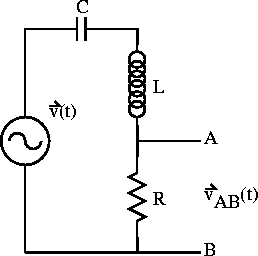
Figure 2.7: Driven series RCL circuit.
Lets now consider putting a sinusoidal source in our series RCL circuit and consider the voltage across one of the circuit elements. The resistor for example in figure 2.7

Figure 2.7: Driven series RCL circuit.
Applying Ohm's law ![]() across the
resistor gives (cf. a voltage divider)
across the
resistor gives (cf. a voltage divider)

where ![]() is known as the transfer function in the
frequency domain.
We have changed independent variables from
is known as the transfer function in the
frequency domain.
We have changed independent variables from ![]() to
to ![]() for
convenience.
for
convenience.
We define
![]()
![]() contains all the information needed to characterize
the circuit.
In exponential form
contains all the information needed to characterize
the circuit.
In exponential form
![]()
where
![]()
and
![]()
![]() has a maximum (resonance) given by
has a maximum (resonance) given by ![]() .
Or
.
Or ![]() is the resonant frequency.
is the resonant frequency.
Example: Consider the series LCR circuit (figure 2.8) driven by a voltage phasor.
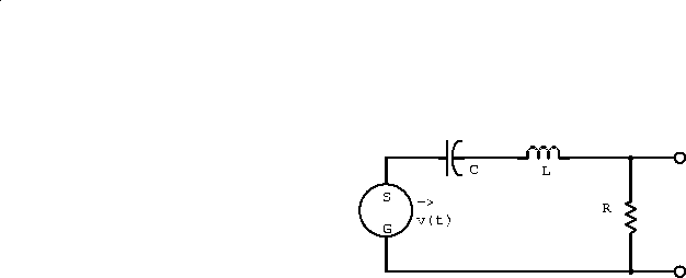
Figure 2.8: Driven series LCR circuit.
- At an angular frequency such that
and
, write the current phasor in terms of
and R.
v(t) is given by v(t)=Zi(t), where
. At
and


Therefore

- At the instant when
is exactly real, calculate the three phasors representing the voltage developed across the R, C, and L circuit elements.
v(t) is real at t=0. Thus

And

Also

- Algebraically and with a sketch on the complex plane, show that the complex voltage sum around the closed loop is zero.
The three voltage phasors are


Around the closed loop
. If this expression is zero at t=0 it will be zero for all time. Therefore
.
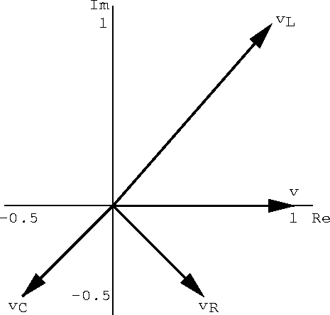
Figure 2.9: Complex voltage sum around the closed loop of the driven LCR circuit.
Example: Sketch simplified versions of the circuit shown in figure 2.10 that would be valid at:
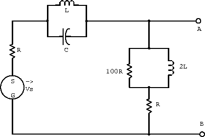
Figure 2.10: Example LCR circuit.
;
.
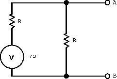
Figure 2.14: Example circuit for.
- very low frequencies but not
;
When
is small
C and L are in parallel and

2L and 100R in parallel gives

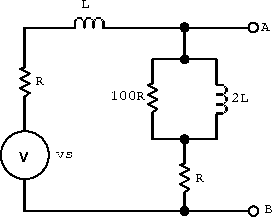
Figure 2.12: Example circuit for very low frequencies but not.
- very high frequencies but not
;
large
(note:
).
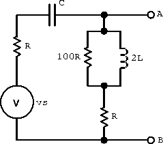
Figure 2.13: Example circuit for very high frequencies but not.
.
.
Example: For the circuit shown in figure 2.15 plotas a function of frequency over the range
rad/s to
rad/s.
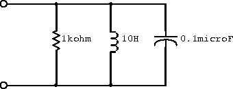
Figure 2.15: Example circuit with components in parallel.
The equivalent impedance for the three components in parallel is

Plugging in the numerical values gives

A table of values and its plot follows.
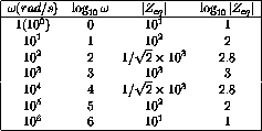
Table 2.1: Numerical values for example circuit.