|
|
|
 |
|
|
|
 |
| |
Outlier Analysis For Cover Type:
The outlier analysis determined that there were a total of two samples within the cover type data set which were greater than 2 standard deviations away from the mean dissimilarity between sites (Figure 1). Upon further inspection, it was found that both sites suffered from an extremely low abundance of all species captured in the data set. These low abundances resulted in a severe lack of similarity to any other sites, causing these sites to be outliers. The outliers were not removed from the data set as the low abundances may be a result of the experimental treatments, and thus I interpreted further analyses with an understanding that these sites should be watched within the analyses. |
|
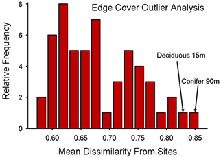
Figure 1: Frequency distribution of mean dissimilarity(Bray-Curtis) from sites and their relative frequency from outlier analysis of cover type data. Treatments which are greater than 2 standard deviations from the mean dissimilarity between sites are indicated by arrows and identified as outliers. |
|
| |
Outlier Analysis for Age Effect:
Within the edge age data set, an outlier analysis again detected two samples which had mean dissimilarities greater than 2 standard deviations from the mean (Figure 2). Looking at the species composition of these sites, I again found that both outlier sites had extremely low abundances of all species. These low abundances resulted in a higher dissimilarity with other sites than might have been expected, and are an important consideration in further analyses. The sites were not removed from the data set however because they may have been a result of the experimental design. In addition, the outliers were not too far outside of the frequency distribution, and thus I decided they should be included (Figure 2). |
|

Figure 2: Frequency distribution of mean dissimilarity(Bray-Curtis) from sites and their relative frequency from outlier analysis of edge age effect data. Treatments which are greater than 2 standard deviations from the mean dissimilarity between sites are indicated by arrows and identified as outliers.
|
|
| |
|
|
|
|
 |
|
|
 |
 |
|
|
|
|
|
|
|
| |
Cover Type Data Checking:
In order to assess the relative data structure, as well as determine any univariate outliers, I calculated the mean species abundance and the standard error within each treatment and cover type. I calculated these descriptive statistics for the total species abundance (all species combined) as well as the three most abundant species within the data set. Looking at the total species abundance (Figure 1), we see that the abundance data takes on a bimodal like distribution along the edge gradient. We also notice that the standard errors are generally consistent along the edge gradient with the exception of the coniferous 15 meter and 105 meter treatments (Figure 1). Thus it is worth considering the relative impact of these treatments in later analyses.
Within the individual species comparisons we see a variety of responses to the edge gradient. Pterostichus adstrictus possesses its greatest abundance in open habitat sites and dropping off farther along the gradient (Figure 2). This species appears to have a unimodal type response to the edge gradient and has low variability between the replicates as is indicated by the small error bars (Figure 2). Calathus advena, an intact forest specialist appears to exhibit a bimodal type response to the edge gradient (Figure 3). The overall low abundances within the deciduous treatments is to be expected as this species is most commonly found within conifer forests. There appears to be a high degree of variability between the replicates as is indicated by the large standard error bars thus consideration should be given to this when interpreting the results (Figure 3). Calathus ingratus had a very different overall distribution with its highest abundance within the deciduous 15 meter site (Figure 4). Based on the pattern of the abundances along the gradient, as well as the larger standard error bars for this treatment, it may be an outlier species and its impact on the analyses should be investigated Figure 4).
|
|
| |

Figure 1: Total pooled abundance of all species along the studied edge gradient. Mean abundances between replciates were determined and standard errors also calculated for each location along the edge gradient. |
|

Figure 2: Mean abundances of Pterostichus adstrictus, an open habitat species along the studied edge gradient. Average abundances between replciates were determined and standard errors also calculated for each location along the edge gradient.
|
|
| |

Figure 3: Mean abundances of Calathus advena , a intact coniferous forest specialist along the studied edge gradient. Average abundances between replciates were determined and standard errors also calculated for each location along the edge gradient. |
|

Figure 4: Mean abundances of Calathus ingratus, the third most common species along the studied edge gradient. Average abundances between replciates were determined and standard errors also calculated for each location along the edge gradient.
|
|
|
|
|
|
|
|
|
|
|
|
| |
Age Effect Data Checking:
I again determined the relative data structure as well as any univariate outliers by calculating the mean and standard errors of species abundances along the edge gradient. Once again these descriptive statistics were calculated for the total species abundances, and the abundances of the three most common species. Within the total pooled species abundances, we see a similar bimodal type pattern in all of the studied edge ages (Figure 1). Although we would have expected the 2 year old clear-cut to have the dominant abundance as it is the most open habitat, in fact we see that the 15 year old clear-cut has the highest abundance (Figure 5). However the high variability of this treatment suggests this mean is driven by a single replicate. The remaining patterns demonstrate a reduction in the relative abundances over time with an increasingly linear patterns the edges age (Figure 5).
The individual species responses to the edge gradient were again variable between species. Pterostichus adstrictus, an open habitat species again has the greatest abundance in the clear-cut and into the 0 meter treatments (Figure 6). This pattern appears to linearize over time, and variances between replicates as demonstrated by the standard errors appears to be low for all treatments (Figure 6). Platynus decentis exhibited a bimodal type response to the edge gradient, with particularly high abundances in the 15 year old clear-cut treatments (Figure 7). This 15 year old clear-cut treatment however had high variability and the average was driven by a single replicate. The remaining abundance patterns appear to be consistent between years and do not seem to change with time (Figure 7). Calathus ingratus also had a high abundance within the 15 year old clear-cut sights, however once again had high variability and was the result of a single replicate driving the mean (Figure 8). The overall pattern in this species abundances was unimodal to bimodal, and again was relatively consistent between years with slight signs of linearization in the 8 year old edge gradient (Figure 8).
|
|
| |

Figure 5: Total pooled abundance of all species along the studied edge gradient. Mean abundances between replciates were determined and standard errors also calculated for each location along the edge gradient. |
|

Figure 6: Mean abundances of Pterostichus adstrictus, an open habitat species along the studied edge gradient. Average abundances between replciates were determined and standard errors also calculated for each location along the edge gradient. |
|
| |
 Figure 7: Mean abundances of Platynus decentis , the second most common species along the studied edge gradient. Average abundances between replciates were determined and standard errors also calculated for each location along the edge gradient. Figure 7: Mean abundances of Platynus decentis , the second most common species along the studied edge gradient. Average abundances between replciates were determined and standard errors also calculated for each location along the edge gradient.
|
|
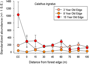
Figure 8: Mean abundances of Calathus ingratus, the third most common species along the studied edge gradient. Average abundances between replciates were determined and standard errors also calculated for each location along the edge gradient.
|
|
|
|
|
|
|
|
|
|
|
|
|
|
|