ECOLOGY OF SPIDERS IN THE BOREAL FOREST
Conserving by Emulating Natural Disturbances
DATA PREPARATION
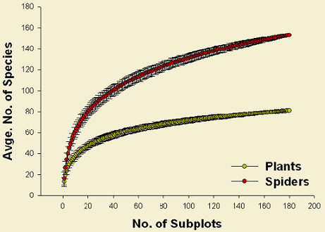
Species area curves for both plant and spider collections were plotted using PC-ORD 5 (McCune & Mefford 2006) to evaluate the suitability of sample size. The average number of species for plants show a tendency to a plateau whereas for spiders tends to continue increasing when reaching 180 subplots (traps). Although this is an indication that sampling effort for spiders was not enough, the data collected is representative for the ground-dwelling assemblage. It can be observed that the accumulation curve seems to start leveling off by the end. In addition, observed species richness (153spp.) correspond in average to more than 80% of estimated richness(ICE: 192 spp., Chao1: 181 spp., Chao2: 184 spp.). These estimations were obtained using EstimateS 7 (Colwell 2006)
The results from this analysis show that for the spider data set 4 of the 60 sites and 2 of the 154 species were outliers. Similarly, for the plant data set, 5 sites and 4 species were outliers. After transforming the data, a second outlier analysis was carried out, showing the same results. The species were removed from the matrices and a new analysis was performed, showing no outliers for the sites. Consequently, this data set was used for the analyses.
It is important to detect outliers in the data set even though multivariate methods are robust for non-normal distributions. As a consequence, an Outlier Analysis was performed using PC-ORD5 (McCune & Mefford 2006), for both rows (sites) and columns (species). This analysis first calculates an average distance between each entity in the matrix with all others, then a frequency distribution of these distances is made and outliers detected from a selected cutoff standard deviation.
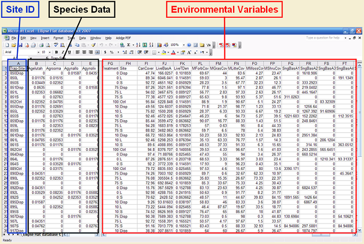
The resulting flat data base contains all the information in the format sites x (species + environmental variables) (rows x columns). Species names were coded for the four first letters of the Genus and Species (Pardosa makenziana = Pardmack). Similarly, all column and raw names were formatted to have only eight characters, thus allowing to be read by different packages. The following image shows and example of this data base:
On the other hand, plant data can't be analyzed as abundance based since the information collected form the plots was percentage cover. Thus, species records on each site correspond to the average percentage cover for the three plots. This average value was log transformed (Log(n+1)), all analyses use this transformed average value.
It is well known that spider assemblages vary during the year, some species are very common and abundant late in the spring but rarely collected as adults later in the summer. Similarly, other species show the opposite trend, and are very common mid/late summer. Thus, one single collection will not be enough to have the best understanding of the effects of harvesting or disturbances over the whole ground-dwelling spider assemblage and conclusions are only partial. To account for this variability, spiders were collected in four different times during the ice-free season: 1. late spring, 2. early summer, 3. mid summer, and 4. late summer.
As a consequence, analyses are carried out and conclusions drawn from the pooled data from these four collections. However, raw spider abundance data can't be used, since throughout the summer some traps were damaged, mainly by vertebrates. By the end of the sampling season, each trap should have operated in the ground for 85 days, but due to animal disturbance, on average the number of days decreased to 74.16. Thus, sampling effort is different and comparisons between sites could be biased for those where less traps were damaged. For this reason, raw abundance was standardized to number of individuals per trap/day to account for uneven sampling. Thus, standardized abundance was calculated for each trap pooling the number of individuals of each species collected by the end of the summer divided by the number of days that the trap operated. Since there were three traps per site and these were not independent, the standardized abundance of these traps was pooled to obtain a single value for each site, thus avoiding the problem of pseudoreplication (Hurlbert, 1984). All analyses were carried out using this value.
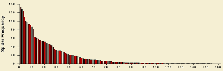
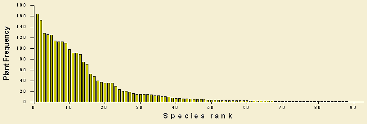
Frequency pots for both plant and species assemblages, show a typical distribution where only few species are very common and a high number of species are found in only few samples. This frequency distribution is strongly skewed to the left and due to the numerous variables associated to each sampling site influencing so many species, multivariate techniques are more suited for analyzing this complex data base. In the Data Analysis section different statistical tools are described.