Analysis

MRT is a technique appropriate for exploring, describing and predicting relationships between multiple species and environmental variables (De'ath 2002). This technique creates hierarchical clusters of sites based on environmental variables, representing species assemblages associated to those environmental variables. Thus, species variability in sites/plots that is explained by similar environmental features is described as a branch in the tree. This technique is very useful, since no assumptions should be met, such as linearity between species and enviroment.

In addition, an Indicator Species Analysis (ISA) (Dufrene & Legendre, 1997) was carried out. This purpose of this method is to asses the value of a species or group of species as indicators for environmental variables. This method is based on the concentration of abundance of a species and its occurrence in a particular predefined group. Thus, the indicator value (IV) is calculated from the relation between the proportional abundance of a species in a particular group and the proportional frequency of this species in the group. When a species is consistently abundant and common in a predefined group, the IV is high in comparison to that in species that are not consistently more associated to the group. A statistical significance is evaluated through a randomization method by testing the IV of both the randomized and non-randomized sets to test the null hypothesis of no difference of IV from chance.

NMS Ordinations performed with the spider and plant assemblages collected at the EMEND landscape, were obtained using PC-ORD 5.1 (McCune & Mefford 2006). From the grouping variables used in the ordination, a Multi-Response Permutation Procedure (MRPP) was carried out. This analysis is a statistical tool to perform pair-wise comparisons between groups that are defined a priori (e.g. forest cover type, harvesting treatment and retention type), for testing the hypothesis of no difference between group levels. This procedure is very useful since no assumptions should be met, such as multivariate normality and homogeneity of variances.

Generally community data is characterized by few common species and a high proportion of rare or uncommon species, generating an incredibly high amount of zeros in the matrix, this is known as the zero-truncation problem (Beals 1984). Since NMS is iterative and is based on ranked distances, this problem is relieved. On each iteration the relationship between the reduced ordination space and the original multidimensional space is enhanced, this iteration process stops when the relationship is minimized, which is measured by a stress value (McCune & Grace 2002); the lower the stress value is, the better the distances in the ordination correspond to the dissimilarity values (Jongman et al. 1995). Ordinations with stress values below 20 are a good representation of the dissimilarity distance matrix and the resulting axes are explaining most of the variation (Clarke 1992, McCune & Grace 2002).

NMS, first suggested by Shepard (1962a, 1962b), is an ordination technique that has been shown to be very appropriate for analyzing community data (Clarke 1992, McCune & Grace 2002), even though it has been widely criticized (Kenkel & Orloci, 1986, Kenkel, 2006). This technique is based on the ranking of distance dissimilarities than the actual distance values, as a consequence NMS needs no assumptions (e.g. multivariate normality, linear relation between species and environment), and also has the flexibility of using any kind of distance to calculate dissimilarities (e.g. Eculidean, Sorensen, Chi-squared). However, to optimize ordination configuration, NMS is computing and time constrained, especially when analyzing large matrices.

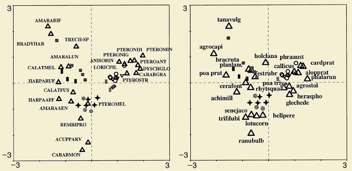
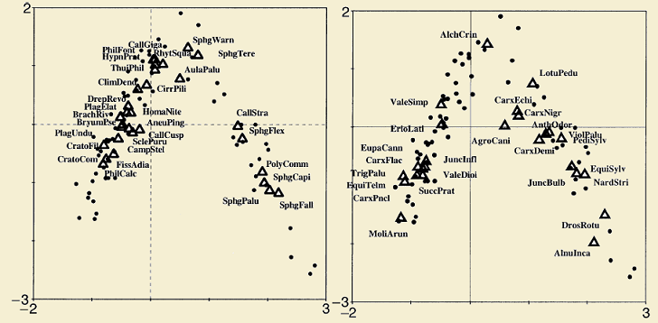
Below, two examples extracted from (ter Braak & Schaffers 2004) are shown. In the first example, beetles and plants were collected from roadside verges in the Netherlands; in the second example, bryophytes and vascular plants were collected from Carphatian spring meadows. This analysis can be calculated in two ways, one (symmetric) to see how related both communities are and other way (predictive) to see how one community is a good predictor for the second.

In both ways, eigenvalues and Inertia (variation explained) for both community assemblages is calculated. In the symmetric way, the species scores of community X are weighted averages of sites scores of community Y, and vice versa (species scores of community Y are weighted averages of sites scores of community X). On the other hand, in the predictive way, species scores are regression weights of both matrices and the site scores are weighted averages of the species scores.This analysis allows to run a predictive CO-CA, in order to establish how predictable is one community (bryophytes) from other community (vascular plants)

For the spider and plant data collected at the EMEND landscape, a CO-CA was carried out including all the observed species. The result from the latter showed a very messy situation, since there were a high number of species in both communities. For reducing this problem and increasing the interpretability of the analysis only the most important species in both communities were included. The way these species were selected, was running consecutive MRT's removing on each step one species at a time, starting from the less abundant species to the more abundant ones. The same trees were consistently obtained until leaving 30 spider species and 48 plant species, beyond this number of species trees started to show differences compared to the tree obtained using all the species. From this procedure, it was concluded that both community assemblages were driven by a certain number of species, the most common ones.

In the examples above species are represented by triangles and sites by dots; for the beetle and plant example, sites are represented by different figures according to site characteristics. Both communities in the examples show a similar pattern in the ordination space suggesting that the community of interest (beetles and bryophytes) are better explained by the plant species composition than to the vegetation structure.

The Co-Correspondence Analysis is an ordination method that relates two types of community assemblages (in this case spiders and plants) sampled from common sites (ter Braak & Schaffers 2004). The main purpose of this ordination technique is to establish in a direct way how two community assemblages are related to each other in order to use one of them as a predictor for the other. It is different from other ordination procedures, for example Canonical Correspondence Analysis (CCA), which predicts one community using the variables that shape a different, but related, community (ter Braak 1096).

As it was mentioned before, there are numerous variables that are associated to a same sampling location. Thus, number of species of different groups (spiders/plants), abundance/%Cover of these species, types of forest, harvesting treatments and associated environmental variables are measured in one single site. As a consequence, multivariate techniques are more appropriate for analyzing this complex scenario.

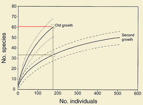
Individual-based rarefaction curves can be used to compare estimated species richness between two or more sites/treatments under the same sampling effort (number of individuals collected). In the example shown on the right (from Colwell et al. 2004), second growth accounted more than 500 individuals whereas in old growth less than 200 individuals were collected. Thus, if richness in these two sites is compared using the total number of samples, old growth would have about 10 more species than second growth. But, when compared under the same sampling effort (about 180 individuals, since it is not known how many species would be present in old growth sites when collecting the same number of individuals as in second growth), it is clear that old growth supports a much higher species richness than second growth.

Different methods are available for measuring species diversity (Magurran 2004). Some of the most common and widely used are the Shannon-Weiner, Simpson's and Fisher's α indices, among many others (Magurran 1998). However, these indices are not very intuitive and sometimes difficult to interpret. As a consequence, taxon sampling curves (species accumulation and rarefaction) are becoming more extensively used due to their advantages: 1. number of species can be standardized to a sample size, 2. estimates of species richness are based on the number of individuals, providing a way of measuring diversity and 3. it is possible to know the rate of accumulation of new species, providing information on sampling effort (Buddle et al. 2005). In addition, taxon sampling curves seem to be more appropriate when analyzing large data sets (high number of samples, individuals and species), which is the case when collecting arthropods.

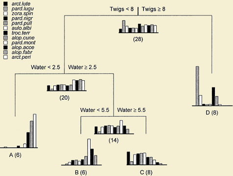
On the right, an example from (De'ath 2002) is shown. The tree represents different clusters of sites with a representative spider assemblage based on some environmental variables. Barplots show multivariate species means at each node with the number of sites in parenthesis. The tree is answering the question of which environmental variables and on what degree these variables are determining the species composition at each site. Two error values are associated to each tree: relative error (RE) and the cross-validated error (CVE). The inverse of RE gives the amount of variance explained by the tree; the CVE gives the power of prediction of new data by the tree.

MRT were carried out for both spider and plant data including all the environmental variables described in the Data Collection section, using the mvpart package in R (De'ath 2007). Trees were selected after obtaining consistently the same tree after 50 trials, the chosen trees were those with the minimum CV-Error. Indicator Species Analyses (description above) were performed using the nodes as grouping variables to determine which species are strongly responding to the more important environmental variables. For an explanation on how to perform MRT in R, click here to visit Josh Jacobs website.

Individual-based rarefaction curves were used to compare species richness and diversity of spiders with the vegan package in R (Oksanen et al. 2007), whereas sample-based rarefaction curves in EstimateS (Colwell 2006) were used for plants. Individual based curves are more suited (Buddle et al. 2005, Colwell et al. 2004), but number of individuals were not recorded for plants, instead percentage cover was estimated, as a consequence only presence/absence estimations can be carried out.

All analyses were performed using the following software packages: