Stand Characteristic Variables
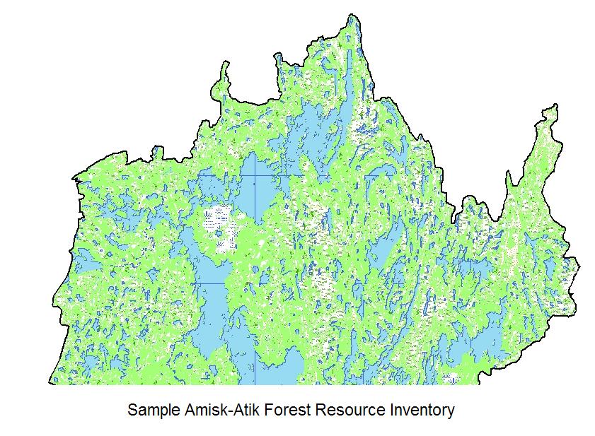
The Amisk-Atik forest resource inventory served as the base for building the data set and provided stand age and species information.
Stand Age
All productive forested polygons in the study area were retained and a stand age was calculated from the "Year of Origin" as listed in the inventory. Although old-growth forest is likely best defined by forest structural stand characteristics (Dunster et al. 1996), stand age was used as a simple indicator of old-growth characteristics for the purpose of the multiple regression analysis.
Tree Species
Similar to stand age, stand composition was also derived directly from the inventory. Five major species were present in the study area: black spruce, white spruce, jack pine, white birch and trembling aspen. The inventory was formatted in a manner that listed three dominant species (SP10, SP11 and SP12) as well as two secondary species (SP20 and SP21). For example, a stand could have an SP10 listed as BS (black spruce) an SP11 of JP (jack pine) and a SP20 of TA (trembling aspen). This would indicate that the stand would be dominated by black spruce with jack pine as a co-dominant and a secondary component of trembling aspen.
In order to convert this information into a quantifiable format that would be suitable for statistical analysis, a separate variable was created for each species. A value from 0-5 was assigned to each polygon to reflect the component of that particular species in the stand. Each species variable had a integer value of 0-5 assigned to reflect the SP10 to SP21 attributes in the inventory. A value of 0 would be interpreted as complete absence of the species in that particular stand and a value of 5 would be assigned if the species was dominant (SP10).
Landscape Variables
 A grid-cell based digital elevation model (DEM) with a 72-metre resolution was used to assign topographic information to
each stand in the study area. Among the topographic variables used were elevation, slope and aspect.
A grid-cell based digital elevation model (DEM) with a 72-metre resolution was used to assign topographic information to
each stand in the study area. Among the topographic variables used were elevation, slope and aspect.
Elevation
The grid-cell based DEM possessing an elevation attribute was converted to a point shapefile and a spatial join was used to calculate mean elevation for each stand based on the points that fell within each polygon. For the relatively minor amount of polygons that did not have a point within its boundaries a second spatial join was performed and an elevation value was assigned to these polygons based on the nearest elevation point.
Slope
Using ESRI’s Spatial Analyst extension, the DEM was converted to a percent slope grid. Through this conversion each grid cell in the DEM was assigned a percent slope value. The grid was then converted to a point shapefile and a spatial join was used to calculate mean percent slope for each stand based on the points that fell within the stand polygon. Similar to Elevation, a second spatial join was required to assign percent slope values to polygons that did not have a point within its boundaries.
Aspect
ESRI’s Spatial Analyst extension was used once again to convert the DEM to an azimuth grid. Through this conversion each grid cell in the DEM was assigned a 0-360 azimuth value. The grid was then converted to a point shapefile and a spatial join was used to calculate mean azimuth for each stand based on the points that fell within the stand polygon.
 Similar to
elevation, a second spatial join was required to assign an azimuth value to polygons that did not have a point within its
boundary.
Similar to
elevation, a second spatial join was required to assign an azimuth value to polygons that did not have a point within its
boundary.
The mean azimuth values needed to be converted to a value that could be used in the statistical analysis. An aspect value of 0 was assigned to due south and 1.0 to due north. The aspect value progressively increased as the mean azimuth increased from south to north. Due west and due east were assigned a value of .5.
Distance to Various Water Features
Variables were assigned to each stand polygon in order to represent its distance from a variety of water features on the landscape. The water features used in the analysis were derived from hydrology layers and included large lakes (>500 ha), medium lakes (100-500 ha), small lakes (<100 ha), streams and wetlands.
 In order to calculate the distance from a stand to each particular water feature, polygon centriods were generated.
The polygon centriods represented the gravitational centre of each stand polygon. A spatial join was then used to calculate
the shortest distance from stand centriods to the edge of each particular water feature. This distance information
was then appended to the dataset through the use of a tabular join.
In order to calculate the distance from a stand to each particular water feature, polygon centriods were generated.
The polygon centriods represented the gravitational centre of each stand polygon. A spatial join was then used to calculate
the shortest distance from stand centriods to the edge of each particular water feature. This distance information
was then appended to the dataset through the use of a tabular join.