3Blue1Brown’s Essence of Linear Algebra[1] YouTube series is a must watch for building intuition in linear algebra. This series exposed gaps in my understanding when I first learned it. In undergraduate, I memorized that a matrix is invertible if and only if the determinant is non-zero. Did I ever understand invertibility or the determinant? No!
Everyone who learns linear algebra should watch this series. It won’t solve your questions, but it deepens your understanding and links mathematical concepts to visualizations. A picture is worth a thousand words, as they say; importantly, intuition and rigour work in tandem.
Often in Computer Science, we treat matrices as data structures (2D arrays), but this series emphasizes that matrices are linear transformations. I’ll summarize the key takeaways and explain how they’re important in machine learning. I will continually add to this post, but for more advanced topics see my blog.
What is a Vector?
“Vector” can mean different things depending on who you ask: [1]
Physics View: A vector is an arrow with length and direction.
CS View: A vector is a list of numbers (e.g., [2, 5, 9]). It’s a data structure.
Mathematician’s View: A vector is anything that follows the rules of addition and scaling.
The Geometric Interpretation
Linear algebra is the bridge between the Physics and CS views. We can represent a list of numbers geometrically!
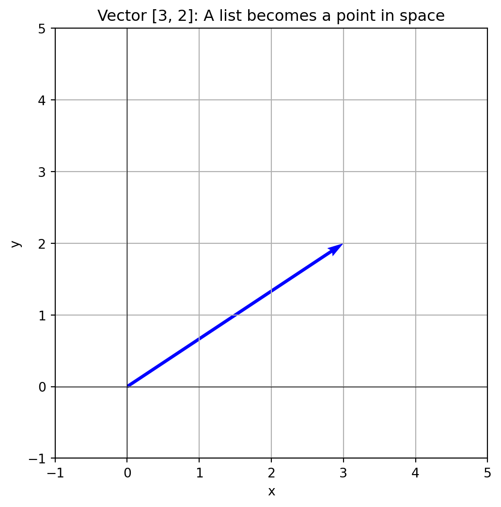
Every vector starts at the origin \((0,0)\):
The x-coordinate is how far you stretch the arrow to the right
The y-coordinate is how far you stretch it up
By doing this, we can represent any list of numbers (CS view) as an arrow in coordinate space (Physics view).
Show code
import numpy as npimport matplotlib.pyplot as plt# The "CS View": Listv = np.array([3, 2])# The "Physics View": Arrow in spaceplt.figure(figsize=(6, 6))plt.quiver(0, 0, v[0], v[1], angles='xy', scale_units='xy', scale=1, color='blue')plt.xlim(-1, 5)plt.ylim(-1, 5)plt.grid(True)plt.axhline(y=0, color='k', linewidth=0.5)plt.axvline(x=0, color='k', linewidth=0.5)plt.title('Vector [3, 2]: A list becomes a point in space')plt.xlabel('x')plt.ylabel('y')plt.show()
Why This Matters for Machine Learning
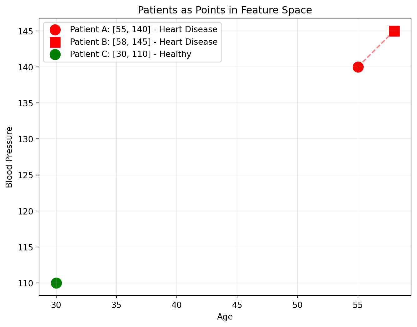
Machine learning learns patterns from data. Each data point becomes a vector, which we can visualize as a point in space!
Example: Imagine you want to predict whether a patient has heart disease. Each patient is described by their measurements:
Age: 55
Blood Pressure: 140
Cholesterol: 250
Heart Rate: 72
The Vector: [55, 140, 250, 72]
Why does this matter? We can measure distance to compare different points:
Two patients that are “similar” (close in space) might have similar health outcomes
A new patient can be classified by looking at their nearest neighbors
This is how ML algorithms like K-nearest neighbors and clustering work
Show code
# Three patients as vectors (using 2 features for visualization)# [Age, Blood Pressure]patient_a = np.array([55, 140]) # Older, high BPpatient_b = np.array([58, 145]) # Similar to Apatient_c = np.array([30, 110]) # Young, healthy BPplt.figure(figsize=(8, 6))plt.scatter(*patient_a, s=150, c='red', label='Patient A: [55, 140] - Heart Disease')plt.scatter(*patient_b, s=150, c='red', marker='s', label='Patient B: [58, 145] - Heart Disease')plt.scatter(*patient_c, s=150, c='green', label='Patient C: [30, 110] - Healthy')# Show distance between A and B (similar patients)plt.plot([patient_a[0], patient_b[0]], [patient_a[1], patient_b[1]], 'r--', alpha=0.5)plt.xlabel('Age')plt.ylabel('Blood Pressure')plt.title('Patients as Points in Feature Space')plt.legend()plt.grid(True, alpha=0.3)plt.show()# Calculate distancesdist_ab = np.linalg.norm(patient_a - patient_b)dist_ac = np.linalg.norm(patient_a - patient_c)print(f"Distance A to B: {dist_ab:.1f} (similar patients, likely similar diagnosis)")print(f"Distance A to C: {dist_ac:.1f} (very different patients)")
Distance A to B: 5.8 (similar patients, likely similar diagnosis)
Distance A to C: 39.1 (very different patients)
Basis Vectors, Linear Combinations, Span, and Independence
\(\hat{i} = [1, 0]\) — points along the x-axis
\(\hat{j} = [0, 1]\) — points along the y-axis
[3, 2]really means: “Take 3 of the \(\hat{i}\) vector and 2 of the \(\hat{j}\) vector and add them up.”
\(\hat{i}\) and \(\hat{j}\) are the basis vectors; the building blocks of our coordinate system.
ML Connection: Your features like Age and Blood Pressure are your basis vectors. If you’re predicting heart disease, \(\hat{i}\) represents “Age” and \(\hat{j}\) represents “Blood Pressure.” Every patient is a combination of these.
What Are Linear Combinations?
There are only two operations allowed in linear algebra: scale vectors (stretch/shrink) and add them together. This “scale and add” process is called a linear combination. Why? Linear algebra deals with lines, and lines that are stretched or added together remain lines.
\[a\vec{v} + b\vec{w}\]
ML Connection: Linear combinations are the foundation of ML models. A linear regression model \(y = w_1x_1 + w_2x_2 + b\) is just a linear combination of feature vectors \(x_1\) and \(x_2\)!
Span and Linear Independence
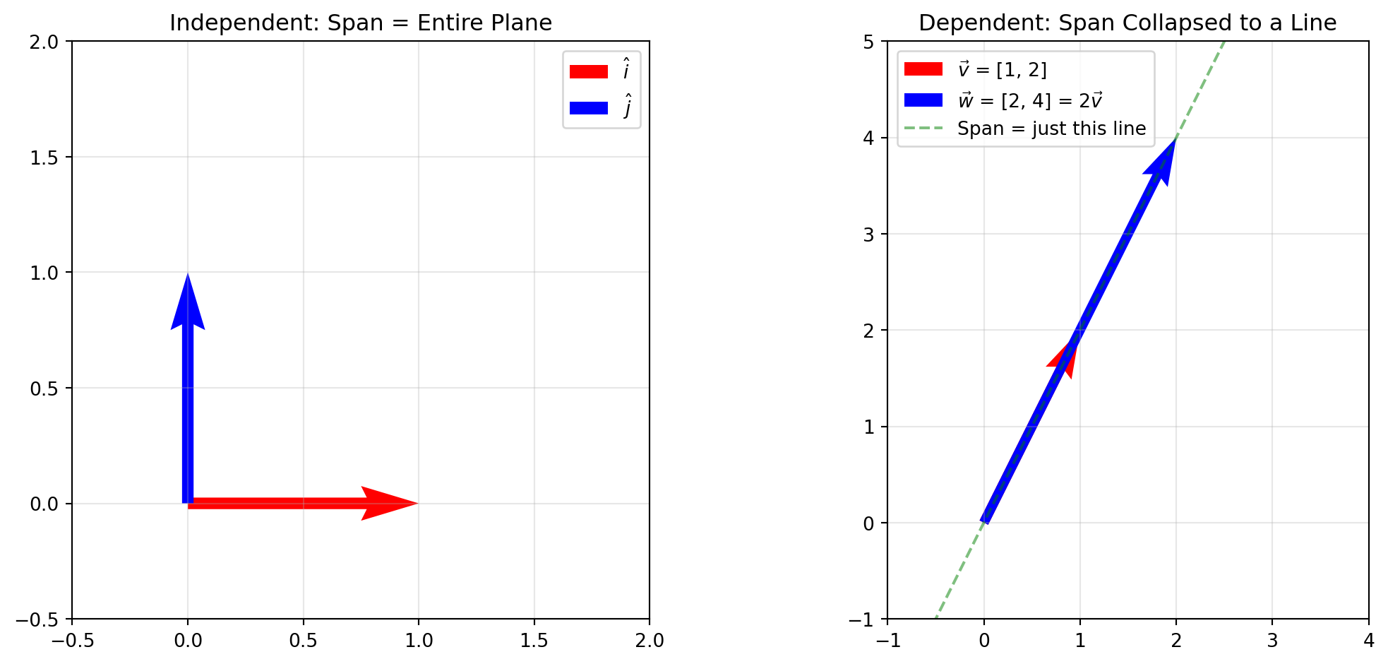
The span is the collection of all points reachable via linear combinations of your basis vectors.
With two vectors, you can usually reach anywhere on the 2D plane. But what if your two vectors point in the same direction? Then you’re stuck on a line and can’t reach the rest of the plane.
Show code
fig, axes = plt.subplots(1, 2, figsize=(12, 5))# Left: Independent vectors span the planeax1 = axes[0]ax1.quiver(0, 0, 1, 0, angles='xy', scale_units='xy', scale=1, color='red', width=0.02, label=r'$\hat{i}$')ax1.quiver(0, 0, 0, 1, angles='xy', scale_units='xy', scale=1, color='blue', width=0.02, label=r'$\hat{j}$')ax1.set_xlim(-0.5, 2)ax1.set_ylim(-0.5, 2)ax1.set_aspect('equal')ax1.grid(True, alpha=0.3)ax1.set_title('Independent: Span = Entire Plane')ax1.legend()# Right: Dependent vectors span only a lineax2 = axes[1]ax2.quiver(0, 0, 1, 2, angles='xy', scale_units='xy', scale=1, color='red', width=0.02, label=r'$\vec{v}$ = [1, 2]')ax2.quiver(0, 0, 2, 4, angles='xy', scale_units='xy', scale=1, color='blue', width=0.02, label=r'$\vec{w}$ = [2, 4] = 2$\vec{v}$')# Show the line they spant = np.linspace(-0.5, 1, 100)ax2.plot(t *3, t *6, 'g--', alpha=0.5, label='Span = just this line')ax2.set_xlim(-1, 4)ax2.set_ylim(-1, 5)ax2.set_aspect('equal')ax2.grid(True, alpha=0.3)ax2.set_title('Dependent: Span Collapsed to a Line')ax2.legend()plt.tight_layout()plt.show()
If one vector can be created by scaling and adding the others, then the vectors are linearly dependent. Notice in the figure above, the second image shows linearly dependent vectors. A set of vectors that are not linearly dependent is linearly independent.
Basis are a set of vectors that are both linearly independent and span the space. They are independent (no redundancy), but can also represent any vector in the space (span)!
ML Connection: In ML, linear dependence is related to information redundancy. In the heart disease prediction example, if you have columns “Weight in kg” and “Weight in lb,” they are linearly dependent because they provide the exact same information. Many algorithms struggle with linearly dependent features.
Matrices Are Linear Transformations
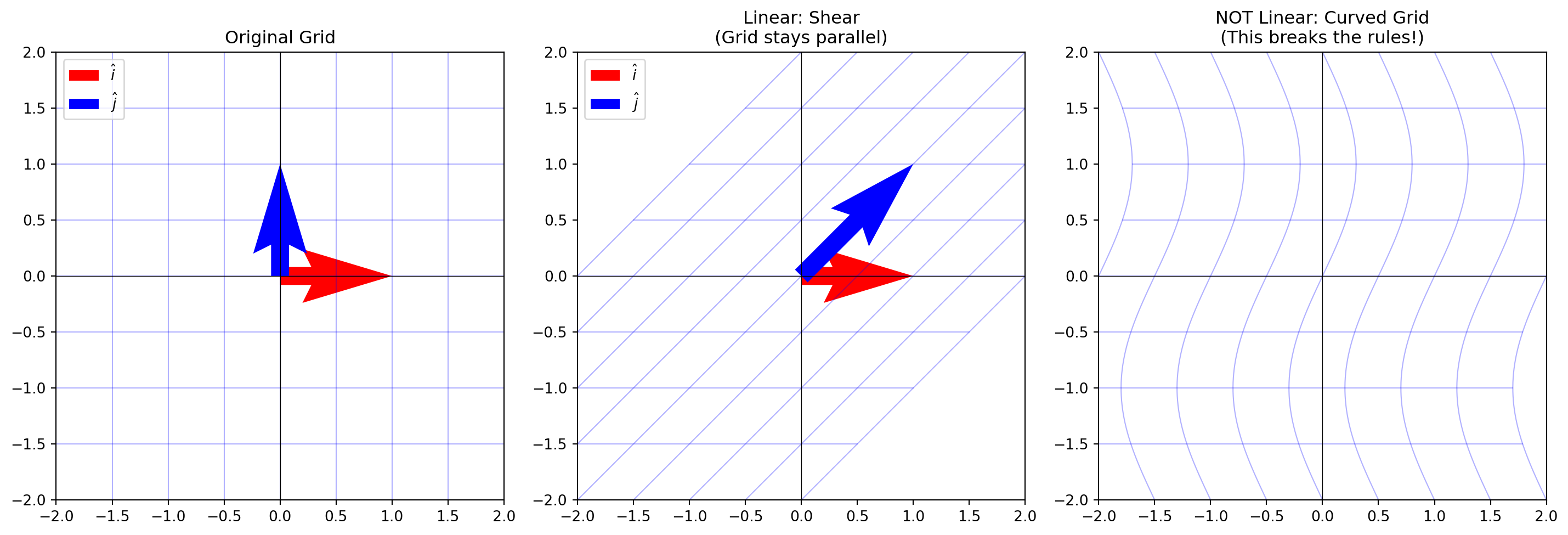
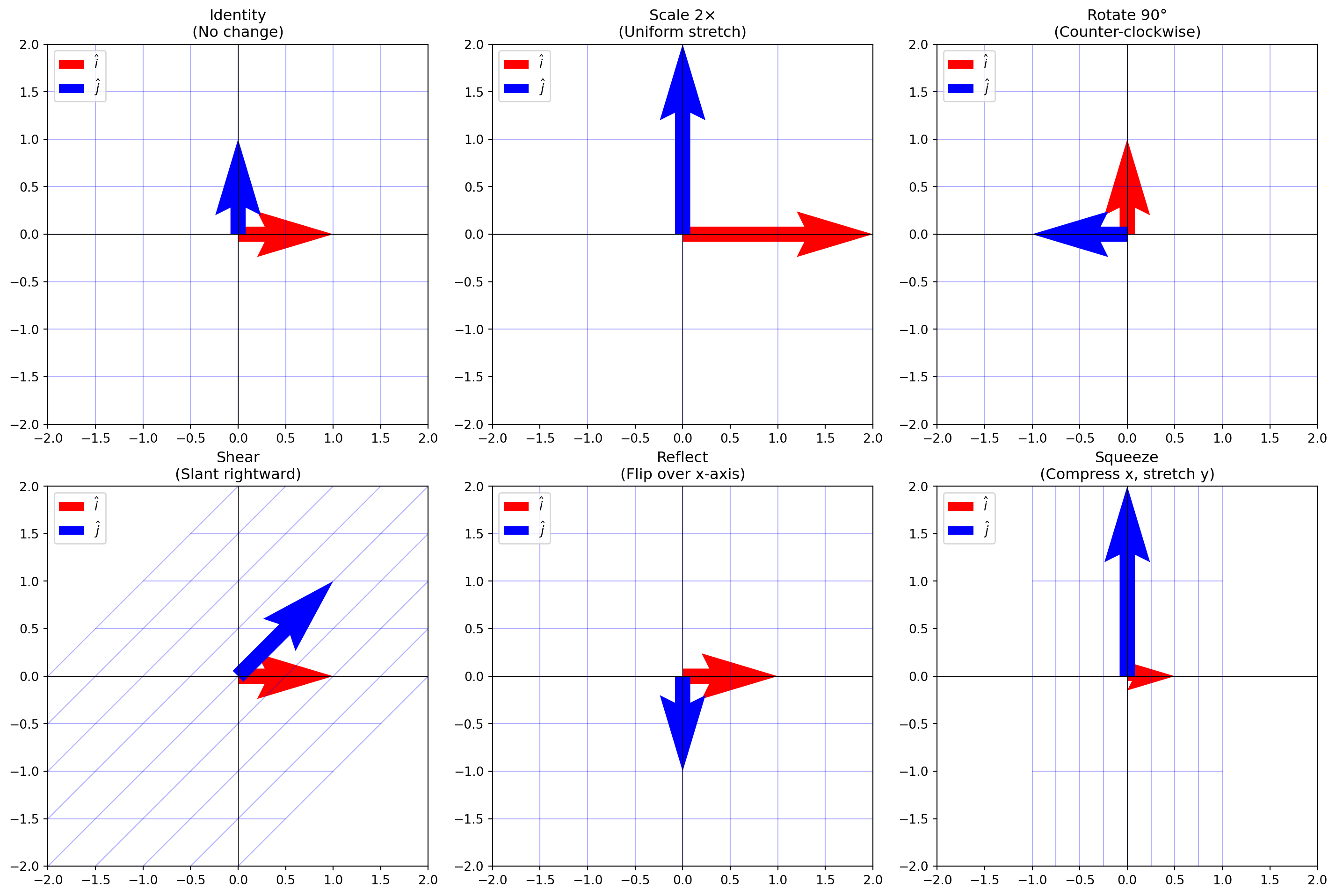
This section emphasizes that matrices are linear transformations (movements). To be a “linear transformation”:
Grid lines must remain parallel and evenly spaced (no curving)
In a neural network, the weights connecting one layer to the next form a weight matrix. Since a matrix is a linear transformation, each layer is really just transforming your data.
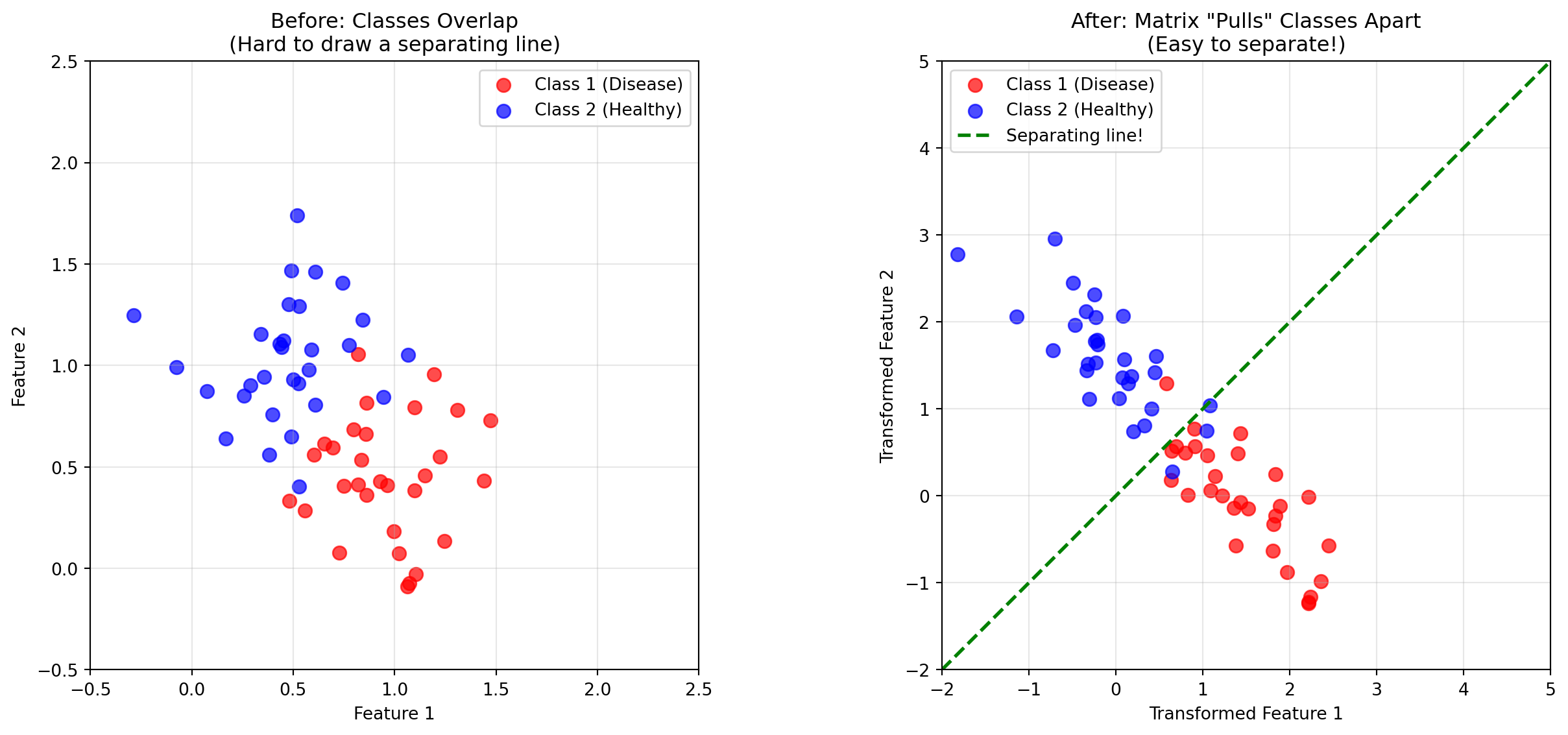
The classic equation you’ll see often in ML is just a linear transformation of your input: \[\text{prediction} = W \cdot \text{input} + b\]
Why? The transformation is trying to separate the data space into recognizable patterns.
Show code
np.random.seed(42)# Generate two classes of points that are NOT linearly separablen_points =30# Class 1 (red): clustered around (1, 0.5)class1 = np.random.randn(n_points, 2) *0.3+ np.array([1, 0.5])# Class 2 (blue): clustered around (0.5, 1)class2 = np.random.randn(n_points, 2) *0.3+ np.array([0.5, 1])# A transformation matrix that separates them better# This stretches along one diagonal and compresses along the otherseparation_matrix = np.array([ [2, -1], [-1, 2]])# Transform the pointsclass1_transformed = (separation_matrix @ class1.T).Tclass2_transformed = (separation_matrix @ class2.T).Tfig, axes = plt.subplots(1, 2, figsize=(14, 6))# Before transformationax1 = axes[0]ax1.scatter(class1[:, 0], class1[:, 1], c='red', s=60, label='Class 1 (Disease)', alpha=0.7)ax1.scatter(class2[:, 0], class2[:, 1], c='blue', s=60, label='Class 2 (Healthy)', alpha=0.7)ax1.set_xlim(-0.5, 2.5)ax1.set_ylim(-0.5, 2.5)ax1.set_aspect('equal')ax1.grid(True, alpha=0.3)ax1.set_xlabel('Feature 1')ax1.set_ylabel('Feature 2')ax1.set_title('Before: Classes Overlap\n(Hard to draw a separating line)')ax1.legend()# After transformationax2 = axes[1]ax2.scatter(class1_transformed[:, 0], class1_transformed[:, 1], c='red', s=60, label='Class 1 (Disease)', alpha=0.7)ax2.scatter(class2_transformed[:, 0], class2_transformed[:, 1], c='blue', s=60, label='Class 2 (Healthy)', alpha=0.7)# Draw a separating lineax2.axline((0, 0), slope=1, color='green', linestyle='--', linewidth=2, label='Separating line!')ax2.set_xlim(-2, 5)ax2.set_ylim(-2, 5)ax2.set_aspect('equal')ax2.grid(True, alpha=0.3)ax2.set_xlabel('Transformed Feature 1')ax2.set_ylabel('Transformed Feature 2')ax2.set_title('After: Matrix "Pulls" Classes Apart\n(Easy to separate!)')ax2.legend()plt.tight_layout()plt.show()
Matrix Multiplication: Composing Transformations
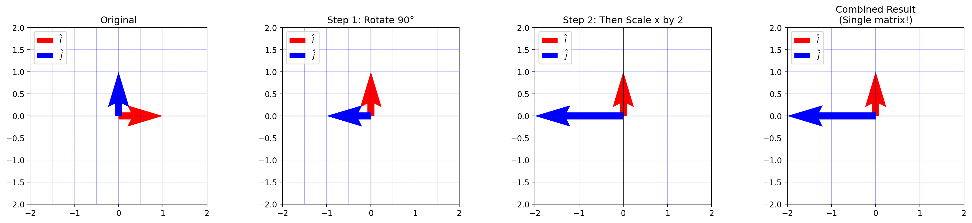
There is a tedious formula for matrix multiplication, but it offers zero intuition. Intuitively, matrix multiplication is not multiplication; it’s a composition of transformations (recall: matrices are transformations).
Multiplying two matrices means applying one transformation (i.e rotation), then applying another (i.e reflection).
The result is a single matrix that represents the combined effect of both transformations.
Show code
# Define the transformationsrotation = np.array([[0, -1], [1, 0]]) # Rotate 90°scale = np.array([[2, 0], [0, 1]]) # Scale x by 2combined = scale @ rotation # First rotate, then scale# Visualize the compositionfig, axes = plt.subplots(1, 4, figsize=(18, 4))plot_grid(axes[0], None, "Original")plot_grid(axes[1], rotation, "Step 1: Rotate 90°")plot_grid(axes[2], scale @ rotation, "Step 2: Then Scale x by 2")plot_grid(axes[3], combined, "Combined Result\n(Single matrix!)")plt.tight_layout()plt.show()
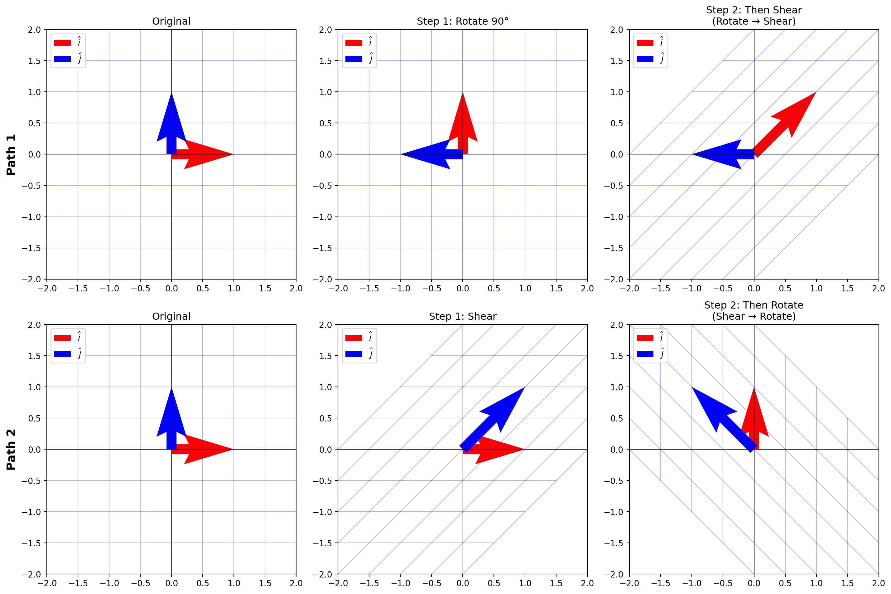
Order Matters!
In school, we learn that \(3 \times 5\) is the same as \(5 \times 3\).
However, for matrices, order matters.\(AB \neq BA\). This is a common bug in ML code!
Show code
# Visual proof: these produce completely different results!fig, axes = plt.subplots(2, 3, figsize=(15, 10))# Top row: Rotate then Shearplot_grid(axes[0, 0], None, "Original")plot_grid(axes[0, 1], rotation, "Step 1: Rotate 90°")plot_grid(axes[0, 2], shear @ rotation, "Step 2: Then Shear\n(Rotate → Shear)")# Bottom row: Shear then Rotateplot_grid(axes[1, 0], None, "Original")plot_grid(axes[1, 1], shear, "Step 1: Shear")plot_grid(axes[1, 2], rotation @ shear, "Step 2: Then Rotate\n(Shear → Rotate)")# Add row labelsaxes[0, 0].set_ylabel("Path 1", fontsize=14, fontweight='bold')axes[1, 0].set_ylabel("Path 2", fontsize=14, fontweight='bold')plt.tight_layout()plt.show()print("Notice: The final grids are different!, ORDER MATTERS!")
Notice: The final grids are different!, ORDER MATTERS!
Notation: We read from right to left.
In the equation \(A(B\vec{x})\):
We transform vector \(\vec{x}\) with \(B\) first, then do a second transformation with \(A\)
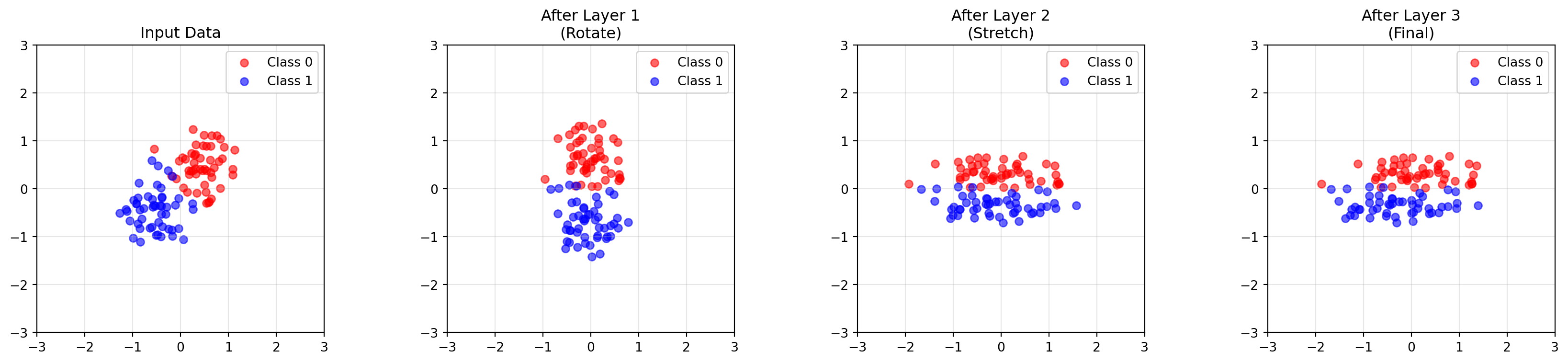
Why This Matters for Machine Learning
This connects to neural networks (a composition of functions). In each layer we could have different weight matrices \(W_1,W_2,W_3,...\) for each layer
The prediction is \(\hat{y} = W_3 \cdot W_2 \cdot W_1 \cdot x\) (ignoring activation functions).
Why? We decompose our problem into a composition of linear transformations.
Show code
# Simulating a simple "neural network" as composed transformationsnp.random.seed(42)# Generate some 2D data pointsn_points =50# Two clusters that need to be separatedcluster1 = np.random.randn(n_points, 2) *0.4+ np.array([0.5, 0.5])cluster2 = np.random.randn(n_points, 2) *0.4+ np.array([-0.5, -0.5])data = np.vstack([cluster1, cluster2])labels = np.array([0] * n_points + [1] * n_points)# "Layer 1": Rotate to align the clustersW1 = np.array([ [0.7, -0.7], [0.7, 0.7]])# "Layer 2": Stretch to separate themW2 = np.array([ [2.0, 0], [0, 0.5]])# "Layer 3": Final rotation for classificationW3 = np.array([ [1, 0.5], [0, 1]])# Apply each layerafter_L1 = (W1 @ data.T).Tafter_L2 = (W2 @ after_L1.T).Tafter_L3 = (W3 @ after_L2.T).T# The composed transformationW_total = W3 @ W2 @ W1after_composed = (W_total @ data.T).Tfig, axes = plt.subplots(1, 4, figsize=(18, 4))titles = ["Input Data", "After Layer 1\n(Rotate)", "After Layer 2\n(Stretch)", "After Layer 3\n(Final)"]datasets = [data, after_L1, after_L2, after_L3]for ax, d, title inzip(axes, datasets, titles): ax.scatter(d[labels==0, 0], d[labels==0, 1], c='red', alpha=0.6, label='Class 0') ax.scatter(d[labels==1, 0], d[labels==1, 1], c='blue', alpha=0.6, label='Class 1') ax.set_aspect('equal') ax.grid(True, alpha=0.3) ax.set_title(title) ax.legend() ax.set_xlim(-3, 3) ax.set_ylim(-3, 3)plt.tight_layout()plt.show()print("Each layer transforms the data to make classification easier.")
Each layer transforms the data to make classification easier.
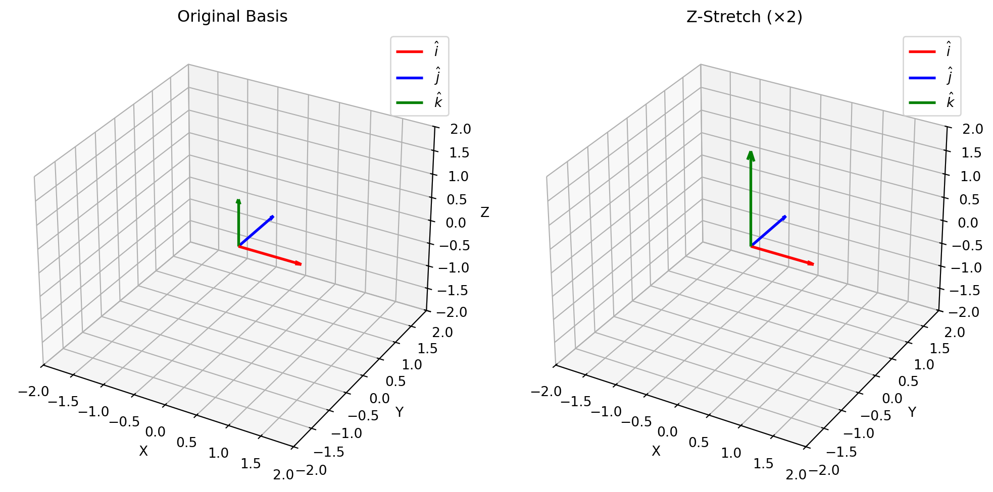
Extending to Higher Dimensions
In 2D, we tracked where \(\hat{i}\) and \(\hat{j}\) landed. In 3D, we can add a third basis vector: \(\hat{k}\) (the z-axis). A \(3 \times 3\) matrix tells us where all three basis vectors land.
ML Connection: ML problems are not 2D or 3D, they’re in much higher dimensions. For example, a \(28 \times 28\) pixel image (like MNIST handwritten digits) is a 784-dimensional vector. Each pixel is a dimension!
We can’t visualize 784 dimensions, but the logic holds when moving to higher dimensions.
A \(784 \times 784\) weight matrix describes where 784 different basis vectors land. Each column tells us where one “pixel direction” ends up after the transformation.
Determinants!
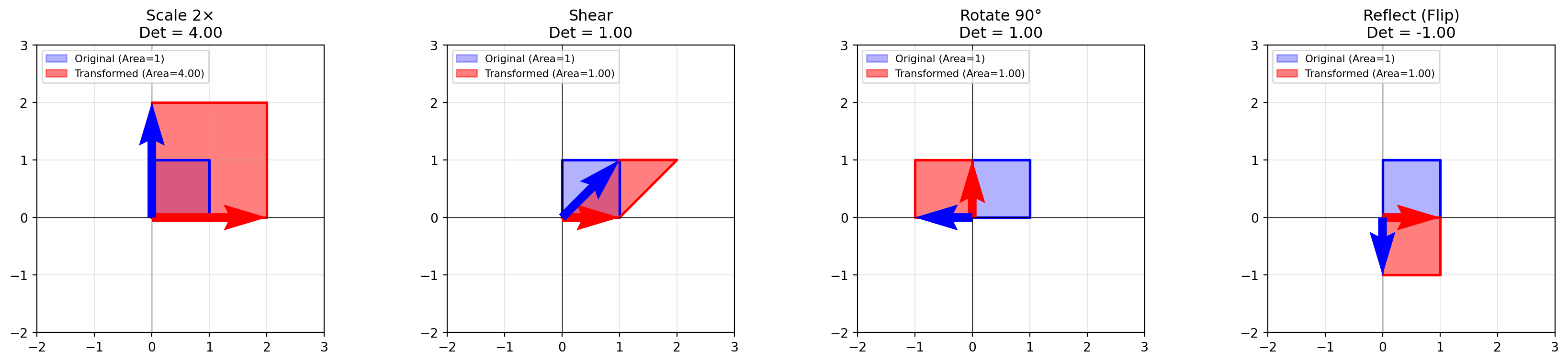
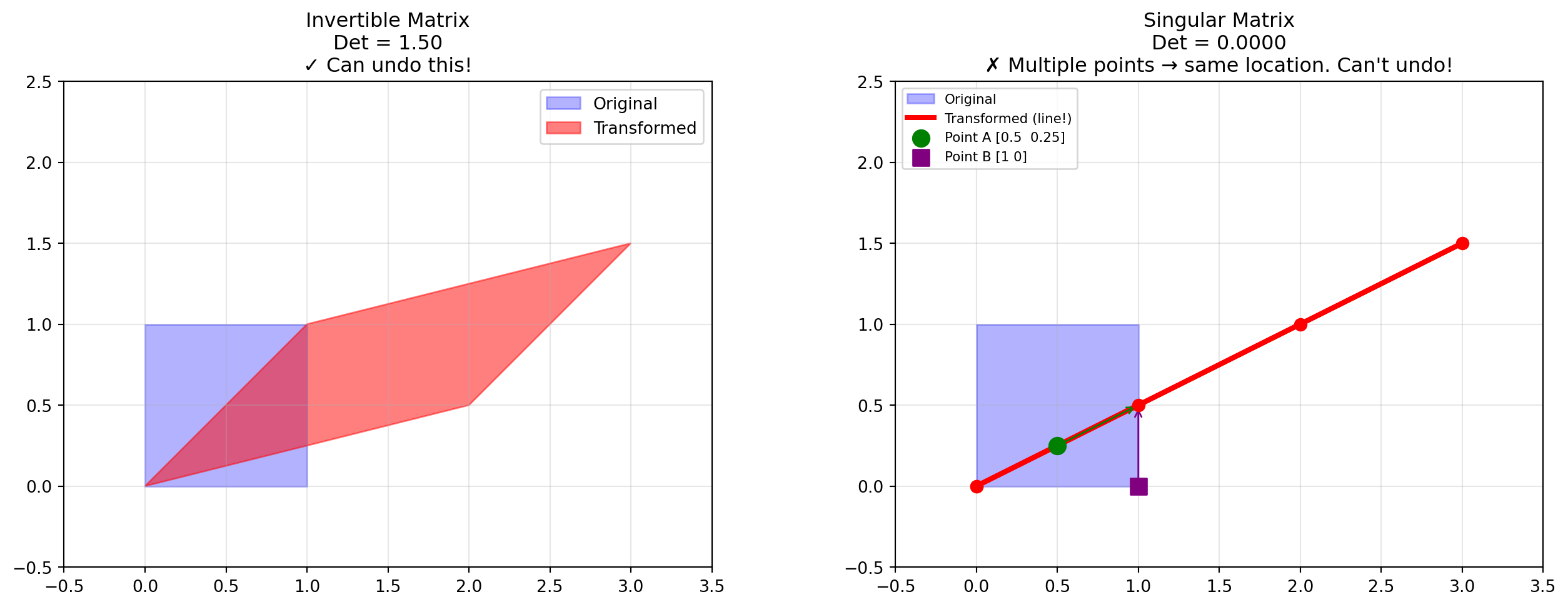
In school, you memorized determinant formulas, but there’s a beautiful geometric meaning: the determinant is the scaling factor by which a transformation changes area.
Take the “unit square” (area = 1) formed by the unit basis vectors. Apply a matrix transformation, it becomes a parallelogram. The area of that parallelogram is the determinant!
If the determinant is 2, the area doubles
If the determinant is 0.5, the area shrinks to half
If the determinant is negative, space has been “flipped”
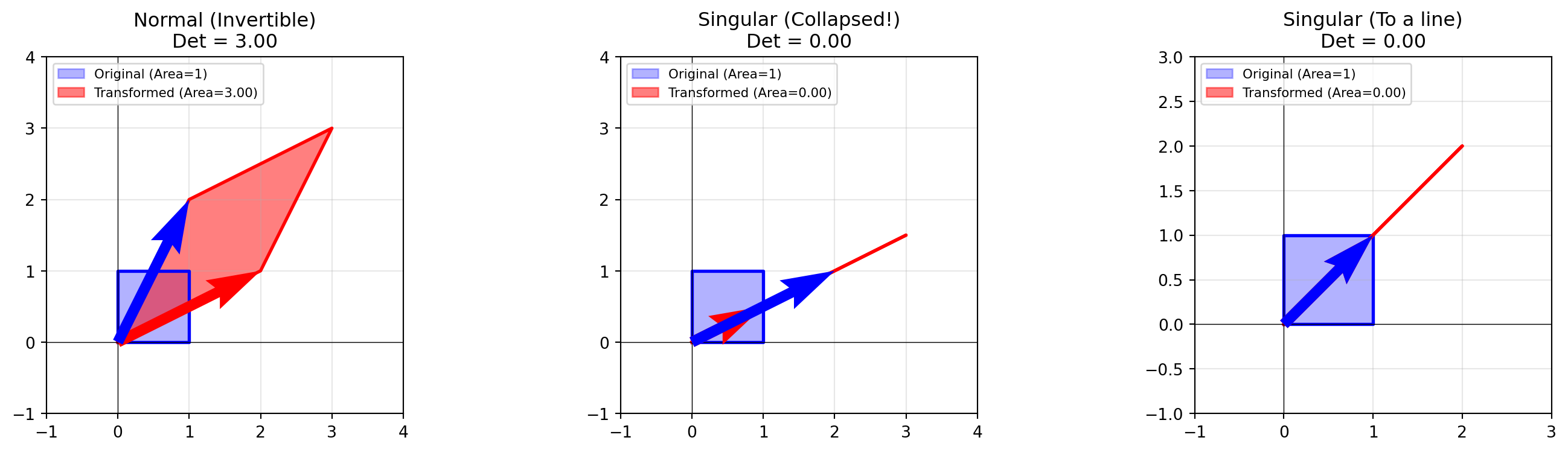
What does it mean if the determinant equals zero? It means you took a 2D square and squished it onto a line (or a point). You’ve lost a dimension! The change in area is 0.
Show code
# Visualize dimension collapsefig, axes = plt.subplots(1, 3, figsize=(15, 4))# Case 1: Normal transformation (det ≠ 0)normal = np.array([[2, 1], [1, 2]])plot_unit_square_transform(axes[0], normal, "Normal (Invertible)")axes[0].set_xlim(-1, 4)axes[0].set_ylim(-1, 4)# Case 2: Collapse to a line (det = 0)singular = np.array([[1, 2], [0.5, 1]]) # Second column is 2× firstplot_unit_square_transform(axes[1], singular, "Singular (Collapsed!)")axes[1].set_xlim(-1, 4)axes[1].set_ylim(-1, 4)# Case 3: Another singular examplesingular2 = np.array([[1, 1], [1, 1]])plot_unit_square_transform(axes[2], singular2, "Singular (To a line)")axes[2].set_xlim(-1, 3)axes[2].set_ylim(-1, 3)plt.tight_layout()plt.show()print("Notice: When det = 0, the 2D square collapses to a 1D line!")
Notice: When det = 0, the 2D square collapses to a 1D line!
Why is it called “Singular”? Once you squish a square into a flat line, you cannot unsquish it back. You’ve destroyed information. The transformation is irreversible. If the determinant is 0, the matrix is not invertible (see the next section). You can’t reverse dimensions! It’s called singular because it uniquely cannot be reversed.
Why This Matters for Machine Learning
1. Information Loss: When the determinant is zero, your matrix has lost information to a lower dimension. Although in ML we want to work with lower dimensions for computation cost, we want to make sure we are not losing important information.
2. Model Crashes: In ML, we often solve equations by inverting a matrix (like the Normal Equation for Linear Regression: \(\theta = (X^TX)^{-1}X^Ty\)). If your determinant is 0, your code will crash because you’re trying to invert a non-invertible matrix.
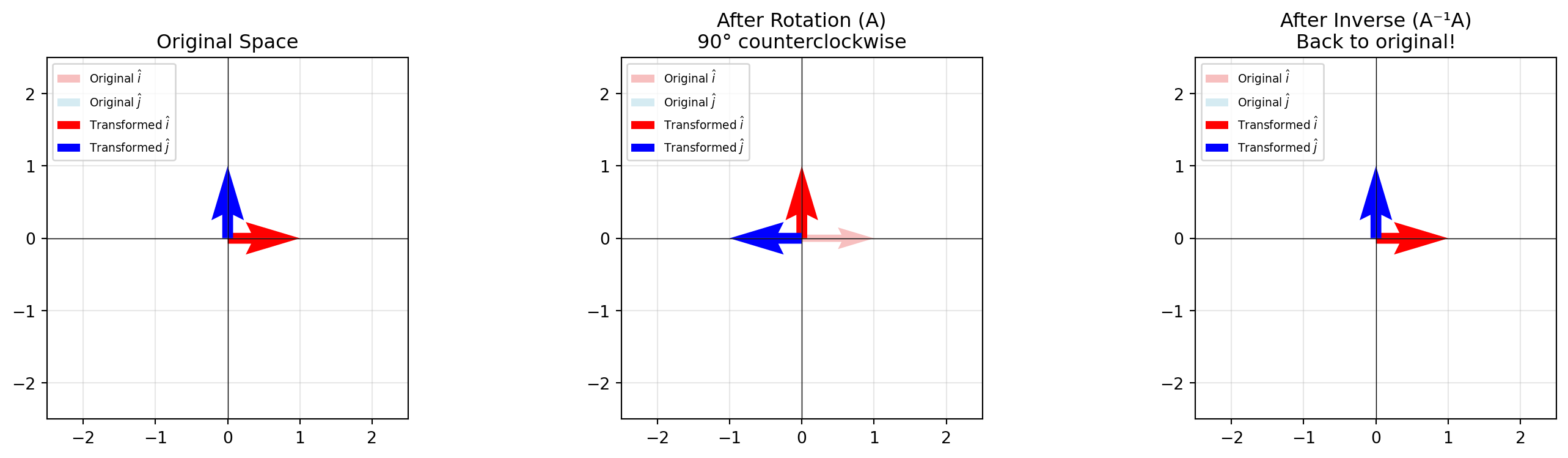
Inverse Matrices, Column Space, Row Space
If a matrix \(A\) is a transformation that moves space (e.g., rotates 90° right), then the inverse matrix\(A^{-1}\) is the transformation that moves it back (rotates 90° left).
Column Space is the span of the matrix columns, all possible outputs of the transformation.
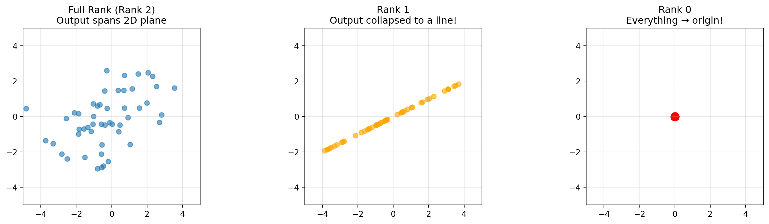
Rank is the number of dimensions in your Column Space.
Full Rank: A \(2 \times 2\) matrix with Rank 2 spans the whole plane. No squishing.
Rank 1: The matrix squishes everything onto a single line.
Rank 0: Everything collapses to the origin.
If your matrix is NOT full rank, then it squishes to a lower dimension, and its not invertible. Thus, your matrix is only invertible when it’s full rank!
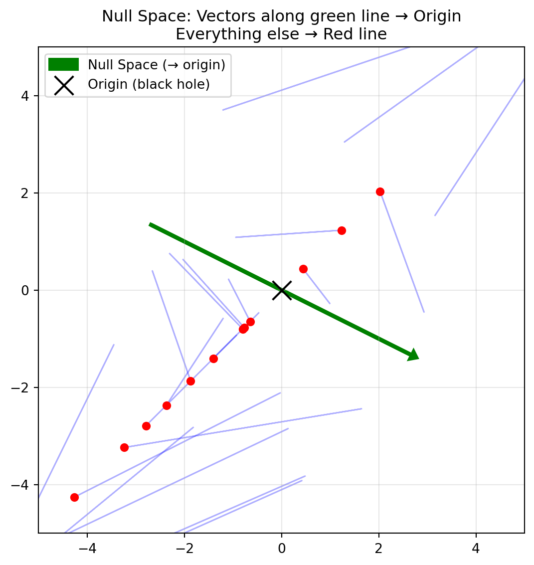
If a transformation squishes dimensions, it forces some vectors to land on zero. The Null Space (or Kernel) is the set of all vectors that get sent to the origin \((0, 0)\).
Since in linear transformation, the origin always stays at the origin, we know the null space contains the origin vector. If we have additional vectors that are in the Null Space, then the dimension shrinks and the matrix is not invertible!
Show code
# Visualize the null spacefig, ax = plt.subplots(figsize=(8, 6))# The matrix squishes everything onto the line y = xA = np.array([[1, 2], [1, 2]])# Plot some input vectors and their outputsnp.random.seed(42)input_vecs = np.random.randn(20, 2) *2for v in input_vecs: output = A @ v ax.arrow(v[0], v[1], output[0] - v[0], output[1] - v[1], head_width=0.1, head_length=0.05, fc='blue', ec='blue', alpha=0.3) ax.scatter(*output, c='red', s=30, zorder=5)# Highlight null space direction (computed directly: [2, -1] normalized)null_vec = np.array([2, -1]) / np.linalg.norm([2, -1]) *3# Scale for visibilityax.arrow(-null_vec[0], -null_vec[1], 2*null_vec[0], 2*null_vec[1], head_width=0.15, head_length=0.1, fc='green', ec='green', linewidth=3, label='Null Space (→ origin)')ax.scatter(0, 0, c='black', s=200, marker='x', zorder=10, label='Origin (black hole)')ax.set_xlim(-5, 5)ax.set_ylim(-5, 5)ax.set_aspect('equal')ax.grid(True, alpha=0.3)ax.legend()ax.set_title("Null Space: Vectors along green line → Origin\nEverything else → Red line")plt.tight_layout()plt.show()
Why This Matters for Machine Learning
Things in ML break when your matrix is not invertible. We now know a matrix is not invertible when it’s not full rank or when the null space contains vectors other than the zero vector.
Regularization (like Ridge Regression) adds \(\lambda I\) to the matrix, artificially restoring full rank:
\((X^TX + \lambda I)^{-1}\)
This makes the matrix invertible again!
Non-Square Matrices
So far, we’ve mostly looked at \(2 \times 2\) matrices (transforming 2D to 2D). But in machine learning, our matrices are rarely square. We usually have many more samples than features, however, the logic doesn’t change!
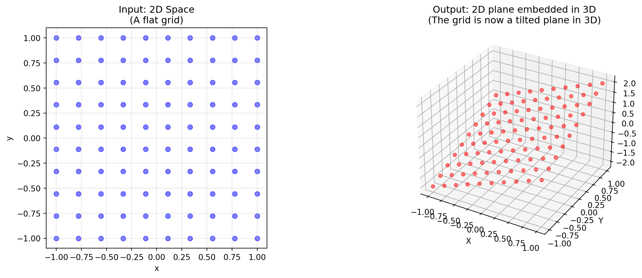
A \(3 \times 2\) Matrix (2 columns, 3 rows):
Input: 2D space (2 columns means it takes 2D vectors)
Output: 3D space (3 rows means it produces 3D vectors)
Visualization: It takes a 2D sheet of paper and embeds it into a 3D room
Rank: The column space is a 2D plane living inside 3D space.
Show code
# A 3x2 matrix: takes 2D input, produces 3D outputM_3x2 = np.array([ [1, 0], [0, 1], [1, 1]])# Generate points on a 2D gridt = np.linspace(-1, 1, 10)grid_2d = np.array([[x, y] for x in t for y in t])# Transform to 3Dgrid_3d = (M_3x2 @ grid_2d.T).Tfig = plt.figure(figsize=(14, 5))# Left: Original 2D spaceax1 = fig.add_subplot(121)ax1.scatter(grid_2d[:, 0], grid_2d[:, 1], c='blue', alpha=0.5)ax1.set_xlabel('x')ax1.set_ylabel('y')ax1.set_title('Input: 2D Space\n(A flat grid)')ax1.set_aspect('equal')ax1.grid(True, alpha=0.3)# Right: Embedded in 3Dax2 = fig.add_subplot(122, projection='3d')ax2.scatter(grid_3d[:, 0], grid_3d[:, 1], grid_3d[:, 2], c='red', alpha=0.5)ax2.set_xlabel('X')ax2.set_ylabel('Y')ax2.set_zlabel('Z')ax2.set_title('Output: 2D plane embedded in 3D\n(The grid is now a tilted plane in 3D)')plt.tight_layout()plt.show()
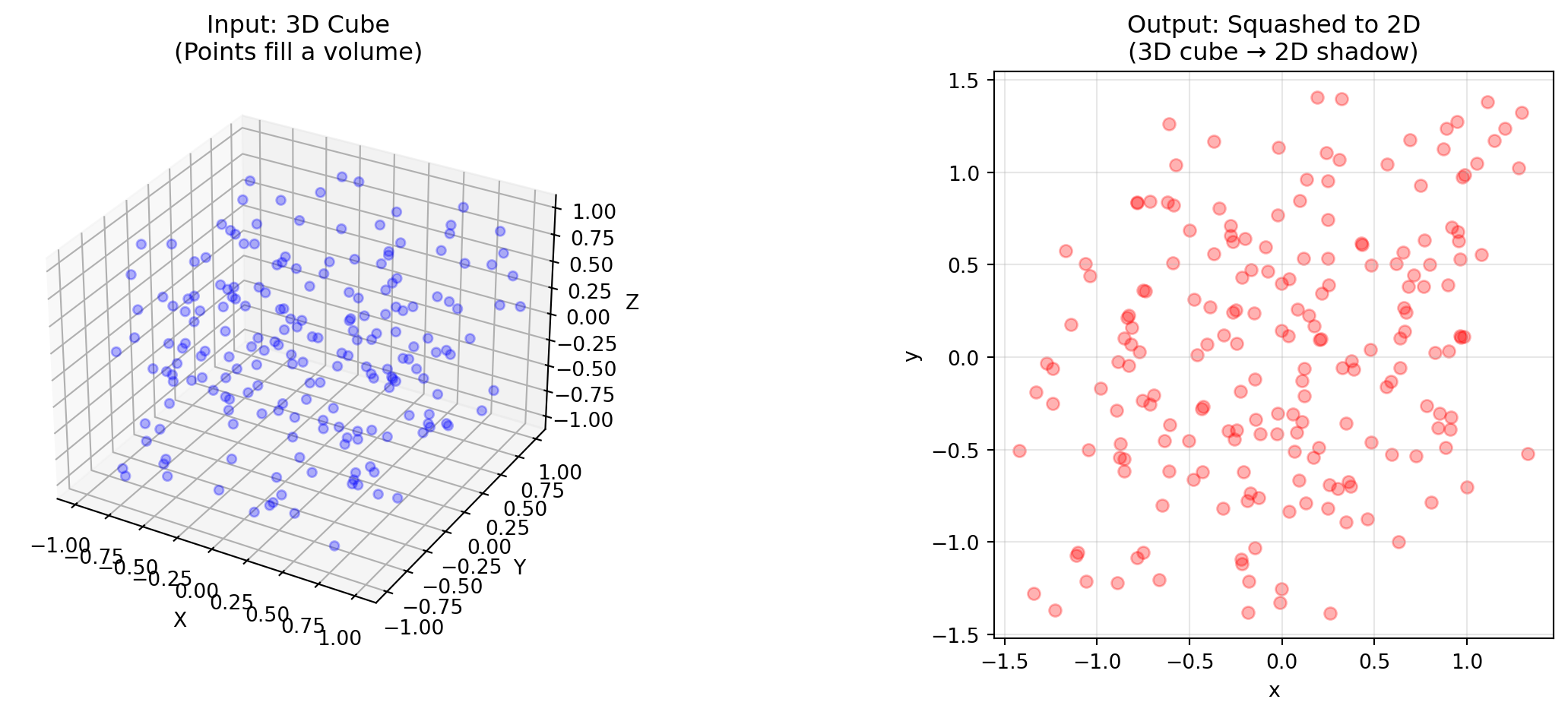
A \(2 \times 3\) Matrix (3 columns, 2 rows):
Input: 3D space (3 columns means it takes 3D vectors)
Output: 2D space (2 rows means it produces 2D vectors)
Visualization: It takes a 3D cube and smashes it onto a flat piece of paper
Rank: It must have a null space! You cannot squeeze 3 dimensions into 2 without destroying at least one dimension of information
Show code
# A 2x3 matrix: takes 3D input, produces 2D outputM_2x3 = np.array([ [1, 0, 0.5], [0, 1, 0.5]])# Generate points in a 3D cubenp.random.seed(42)cube_3d = np.random.rand(200, 3) *2-1# Random points in [-1, 1]^3# Squash to 2Dflat_2d = (M_2x3 @ cube_3d.T).Tfig = plt.figure(figsize=(14, 5))# Left: Original 3D cubeax1 = fig.add_subplot(121, projection='3d')ax1.scatter(cube_3d[:, 0], cube_3d[:, 1], cube_3d[:, 2], c='blue', alpha=0.3)ax1.set_xlabel('X')ax1.set_ylabel('Y')ax1.set_zlabel('Z')ax1.set_title('Input: 3D Cube\n(Points fill a volume)')# Right: Squashed to 2Dax2 = fig.add_subplot(122)ax2.scatter(flat_2d[:, 0], flat_2d[:, 1], c='red', alpha=0.3)ax2.set_xlabel('x')ax2.set_ylabel('y')ax2.set_title('Output: Squashed to 2D\n(3D cube → 2D shadow)')ax2.set_aspect('equal')ax2.grid(True, alpha=0.3)plt.tight_layout()plt.show()
The Dot Product: “Similarity”
The dot product is used a lot in machine learning. The dot product is “element-wise multiplication and addition”:
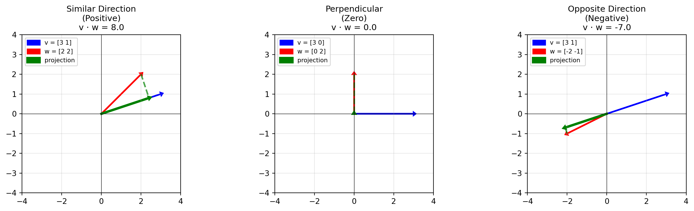
But this doesn’t intuitively tell us what it means and why we like it in machine learning. Geometrically, the dot product is a projection.
Imagine shining a light perpendicular to vector \(\vec{v}\). The “shadow” of vector \(\vec{w}\) falls onto \(\vec{v}\). The dot product is the length of that shadow multiplied by the length of \(\vec{v}\).
Positive: The vectors point in roughly the same direction (“Similar”)
Zero: The vectors are perpendicular (“No Relation”)
Negative: The vectors point in opposite directions (“Different”)
Dot Product in terms of Vectors
Remember non-square matrices? A \(1 \times 2\) matrix takes 2D vectors and outputs a single number (1D):
\[\begin{bmatrix} 2 & 3 \end{bmatrix} \begin{bmatrix} x \\ y \end{bmatrix} = 2x + 3y\]
But wait… that’s exactly the same as a dot product with the vector \(\begin{bmatrix} 2 \\ 3 \end{bmatrix}\)!
Why This Matters for Machine Learning
The dot product = similarity. This powers many ideas in ML.
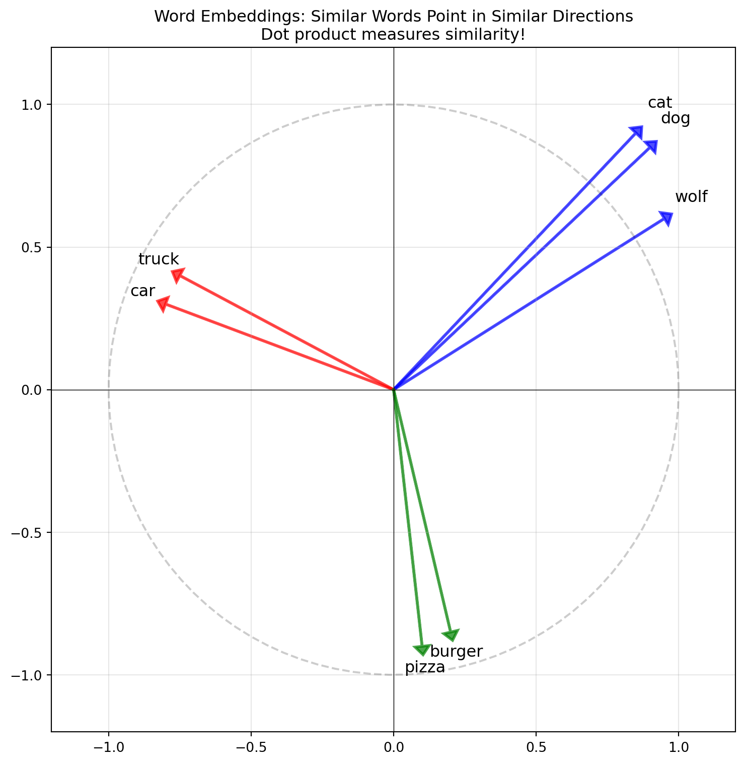
1. Cosine Similarity
One can show using trigonometry that \(\vec{v} \cdot \vec{w} = |\vec{v}||\vec{w}|\cos(\theta)\). With this we can measure how “similar” two vectors are. Since \(\cos(\theta)\) is between \([-1,1]\), the higher the number, the more related they are.
def cosine_similarity(v, w):return np.dot(v, w) / (np.linalg.norm(v) * np.linalg.norm(w))# Visualize in 2D (simplified embedding space)fig, ax = plt.subplots(figsize=(8, 8))# 2D "embeddings" for visualizationwords = {'dog': np.array([0.9, 0.85]),'cat': np.array([0.85, 0.9]),'wolf': np.array([0.95, 0.6]),'car': np.array([-0.8, 0.3]),'truck': np.array([-0.75, 0.4]),'pizza': np.array([0.1, -0.9]),'burger': np.array([0.2, -0.85]),}colors = {'dog': 'blue', 'cat': 'blue', 'wolf': 'blue','car': 'red', 'truck': 'red','pizza': 'green', 'burger': 'green'}for word, vec in words.items(): ax.arrow(0, 0, vec[0], vec[1], head_width=0.05, head_length=0.03, fc=colors[word], ec=colors[word], linewidth=2, alpha=0.7) ax.annotate(word, vec *1.1, fontsize=12, ha='center')ax.set_xlim(-1.2, 1.2)ax.set_ylim(-1.2, 1.2)ax.set_aspect('equal')ax.grid(True, alpha=0.3)ax.axhline(y=0, color='k', linewidth=0.5)ax.axvline(x=0, color='k', linewidth=0.5)ax.set_title('Word Embeddings: Similar Words Point in Similar Directions\n''Dot product measures similarity!', fontsize=12)# Add a unit circle for referencetheta = np.linspace(0, 2*np.pi, 100)ax.plot(np.cos(theta), np.sin(theta), 'k--', alpha=0.2)plt.tight_layout()plt.show()print("=== Word Embedding Similarity ===\n")print(f"Similarity(dog, cat): 0.998, Very similar!")print(f"Similarity(dog, car): 0.256, Very different!")
=== Word Embedding Similarity ===

Similarity(dog, cat): 0.998, Very similar!
Similarity(dog, car): 0.256, Very different!
Cosine Similarity is used in all sorts of applications like in Large Language Models to measure semantic similarity between word vectors and recommendation systems (similar items)!
Eigenvectors and Eigenvalues
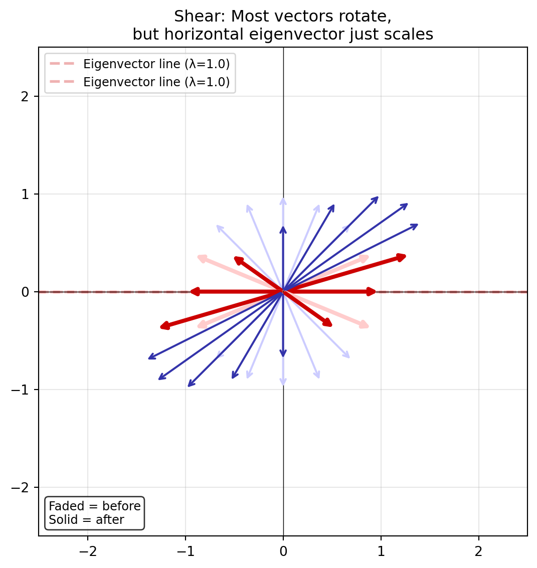
Matrices are linear transformations of vectors. When a matrix transforms a vector, the vector usually changes direction. But there are special vectors that don’t change direction. These are called eigenvectors and are on the same line but only stretched (eigenvalues).
These special vectors are called Eigenvectors.
The amount they stretch is called the Eigenvalue (\(\lambda\)).
Mathematically, this is the equation:
\[A\vec{v} = \lambda\vec{v}\]
The matrix \(A\) acting on vector \(\vec{v}\) is the same as just scaling it by the number \(\lambda\).
Show code
fig, ax = plt.subplots(figsize=(8, 6))def visualize_eigenvectors(ax, matrix, title):"""Show how a matrix transforms many vectors, highlighting eigenvectors."""# Find eigenvalues and eigenvectors evals, evecs = np.linalg.eig(matrix)# Draw many vectors around a circle to show the transformation n_vectors =16 angles = np.linspace(0, 2*np.pi, n_vectors, endpoint=False)for angle in angles:# Original vector on unit circle v = np.array([np.cos(angle), np.sin(angle)])# Transformed vector v_trans = matrix @ v# Check if this is close to an eigenvector direction is_eigen =Falsefor i inrange(len(evals)): evec = np.real(evecs[:, i]) evec_normalized = evec / np.linalg.norm(evec)# Check alignment (dot product close to ±1)ifabs(abs(np.dot(v, evec_normalized)) -1) <0.1: is_eigen =Truebreakif is_eigen:# Eigenvector: red, with clear before/after contrast# Before: dashed outline style ax.annotate('', xy=v, xytext=(0, 0), arrowprops=dict(arrowstyle='->', color='#ffcccc', lw=3))# After: solid bold red ax.annotate('', xy=v_trans, xytext=(0, 0), arrowprops=dict(arrowstyle='->', color='#cc0000', lw=3))else:# Regular vector: blue with clear contrast# Before: light dashed ax.annotate('', xy=v, xytext=(0, 0), arrowprops=dict(arrowstyle='->', color='#ccccff', lw=1.5))# After: solid blue ax.annotate('', xy=v_trans, xytext=(0, 0), arrowprops=dict(arrowstyle='->', color='#3333aa', lw=1.5))# Draw eigenvector lines (the "axes" of the transformation)for i inrange(len(evals)):if np.isreal(evals[i]): evec = np.real(evecs[:, i]) eval_val = np.real(evals[i])# Extend line through origin t = np.linspace(-2.5, 2.5, 100) ax.plot(t * evec[0], t * evec[1], '--', color='#cc0000', alpha=0.3, linewidth=2, label=f'Eigenvector line (λ={eval_val:.1f})') ax.set_xlim(-2.5, 2.5) ax.set_ylim(-2.5, 2.5) ax.set_aspect('equal') ax.grid(True, alpha=0.3) ax.axhline(y=0, color='k', linewidth=0.5) ax.axvline(x=0, color='k', linewidth=0.5) ax.set_title(title, fontsize=12) ax.legend(loc='upper left', fontsize=9)# Add annotation ax.text(0.02, 0.02, 'Faded = before\nSolid = after', transform=ax.transAxes, fontsize=9, verticalalignment='bottom', bbox=dict(boxstyle='round', facecolor='white', alpha=0.8))# Shear matrixshear = np.array([[1, 1], [0, 1]])visualize_eigenvectors(ax, shear, "Shear: Most vectors rotate,\nbut horizontal eigenvector just scales")plt.tight_layout()plt.show()
Notice how most vectors (blue) change direction after transformation, but the eigenvectors (red) stay on their line (they are only stretched)