Turning now from classical mechanics to quantum mechanics, a free photon
can be represented by a wave function ![]() , which satisfies the
equation
, which satisfies the
equation
| (7.97) |
A plane-wave solution to this equation is
| (7.98) |
where
![]() is the four-momentum and
is the four-momentum and
![]() is the unit polarization four-vector of the photon.
We will discuss the polarization and normalization presently.
is the unit polarization four-vector of the photon.
We will discuss the polarization and normalization presently.
On substituting into the equation, we fine ![]() satisfies
satisfies
| (7.99) |
The polarization vector has four components and yet it describes a
spin-1 particle.
The Lorentz condition
![]() , gives
, gives
| (7.100) |
and this reduces the number of independent components of
![]() to three.
Moreover, we have to explore the consequences of the additional gauge
freedom.
Choose a gauge parameter
to three.
Moreover, we have to explore the consequences of the additional gauge
freedom.
Choose a gauge parameter
| (7.101) |
with constant ![]() so that
so that ![]() is satisfied.
This, together with the solution for
is satisfied.
This, together with the solution for ![]() shows that the physics is
unchanged by the replacement
shows that the physics is
unchanged by the replacement
| (7.102) |
In other words, two polarization vectors
![]() which differ by a multiple
of
which differ by a multiple
of ![]() describe the same photon.
We may use this freedom to ensure that the time component of
describe the same photon.
We may use this freedom to ensure that the time component of
![]() vanishes,
vanishes,
![]() ; and then the
Lorentz condition reduces to
; and then the
Lorentz condition reduces to
| (7.103) |
This (noncovariant) choice of gauge is known as the Coulomb gauge.
We see that there are only two independent polarization vectors and
that they are both transverse to the three-momentum of the photon.
For example, for a photon traveling along the ![]() -axis, we may take
-axis, we may take
| (7.104) |
These are referred to as linear polarization vectors. The linear combinations
| (7.105) | |||
| (7.106) |
are called circular polarization vectors.
A free photon is thus described by its momentum ![]() and a
polarization vector
and a
polarization vector
![]() .
Since
.
Since
![]() transforms as a vector, we anticipate that
it is associated with a particle of spin-1.
If
transforms as a vector, we anticipate that
it is associated with a particle of spin-1.
If
![]() were along
were along ![]() , it would be associated
with a helicity-zero photon.
This state is missing because of the transversability condition
, it would be associated
with a helicity-zero photon.
This state is missing because of the transversability condition
![]() .
It can only be absent because the photon is massless.
.
It can only be absent because the photon is massless.
In a special Lorentz frame ![]() is pure space-like,
is pure space-like,
![]() , with
, with
![]() .
In an arbitrary Lorentz frame
.
In an arbitrary Lorentz frame ![]() is space-like and
normalized to
is space-like and
normalized to ![]() .
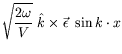
The normalization constant of the plane wave for a photon is chosen
such that the energy in the wave
.
The normalization constant of the plane wave for a photon is chosen
such that the energy in the wave ![]() is just
is just
![]() (ie.
(ie.
![]() for a single photon).
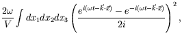
To verify this, we compute
for a single photon).
To verify this, we compute
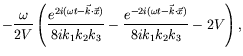
| (7.107) |
This if for the Heaviside-Lorentz system of units.
In the Gaussian system of units the constant in front of the integral
would be ![]() .
Since (
.
Since (![]() in the Lorentz gauge)
in the Lorentz gauge)
 |
|||
 |
(7.108) |
 |
(7.109) |
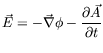
and
| (7.110) |
Thus
![]() and
and
 |
|||
 |
|||
 |
|||
| (7.111) |
where we have taken the time average.
The completeness relationship for polarization vectors is
| (7.112) |