

Method
The numbers of individuals for each sample
unit was estimated using the mean of the number of animals observed in
each transect (10 in each one). Because Region III of “Big HR” had a
number for Linear Disturbance higher than Control, it was removed from
the dataset. It was assumed than an external element affected the data
sampling (e.g. bad weather condition).
Figure 2: RESIDUAL GRAPH
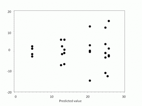
Residual graph for Animal Movement and Landscape Disturbance treatements. Axis X, Predicted value is Individual Number. Axis Y, Residual value.
A residual graph (Fig. 2) was built for
the observed normality tendency and equal variances in the dataset.
This graph illustrated that the dataset had a normal distribution, but
unequal variance.
A Levine’s Test was applied to check the equal
variance on Animal Movement and Landscape Disturbance treatments. The
result showed than Animal Movement had unequal variance (p=0,043),
while Landscape Disturbance had equal variance (p=0,812).
Boxplot
graphs (Fig. 3) were building to visualize the general data
behavior. An ANOVA test and Pairwise Comparisons were applied to
each Animal Movement to assess the impact of Landscape Disturbances
over the number of individuals.
Figure 3: BOXPLOT FOR ANIMAL MOVEMENT AND LANDSCAPE DISTURBANCE VARIABLES.
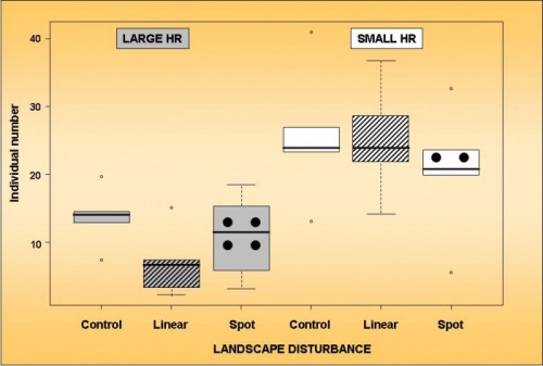
Boxplot
for Animal Movement (Large HR and Small HR) and Landscape
Disturbance (Control, Linear and Spot). Regions were considered as
repetition (for Large HR N = 4 because Region III was eliminated;
for Small N=5).