Classification of simple Lie algebras

Section 5.9 Classification of simple Lie algebras

Objectives

You should be able to:

Sketch the main ideas behind the classification of simple Lie algebras.
State the result of the classification of simple Lie algebras.

In this section we will sketch the main ideas behind one of the most fundamental result in Lie theory, the classification of simple Lie algebras.

🔗

Subsection 5.9.1 Simple Lie algebras

🔗

Recall the definition of simple groups (see Definition 1.9.5): a group is simple if it has no non-trivial (or proper) normal subgroups. It turns out that there is a similar concept of a simple Lie algebra, which we now define.

🔗

Definition 5.9.1. Lie subalgebra.

Let $\mathfrak{g}$ be a Lie algebra. A Lie subalgebra is a subspace $\mathfrak{h} \subset \mathfrak{g}$ that is closed under the bracket. That is, for all $X,Y \in \mathfrak{h}\text{,}$ $[X,Y] \in \mathfrak{h}\text{.}$

🔗

Definition 5.9.2. Invariant Lie subalgebra.

A Lie subalgebra $\mathfrak{h} \subset \mathfrak{g}$ is invariant if for all $X \in \mathfrak{h}$ and all $Y \in \mathfrak{g}\text{,}$ $[X,Y] \in \mathfrak{h}\text{.}$ In mathematical terminology, this is also called an ideal in the Lie algebra $\mathfrak{g}\text{.}$

🔗

The notion of invariant subalgebras is closely connected to the notion of normal subgroups. Indeed, the definition is pretty much the same, with the operation of conjugation for groups replaced by the bracket operation for algebras. Concretely, one can show that invariant Lie subalgebras give rise to normal subgroups of Lie groups by exponentiation.

🔗

Definition 5.9.3. Simple Lie algebra.

A Lie algebra is simple if it has no non-trivial invariant Lie subalgebras. It is semisimple if it is a direct sum of simple Lie algebras.

🔗

This is the algebra counterpart to the notion of simple groups. It turns out that simple Lie algebras are very nice, and in fact can be fully classified. This is what we now turn to.

🔗

Subsection 5.9.2 Construction of the classification

🔗

To classify simple Lie algebras one needs to introduce a number of concepts that we have not discussed yet. We will be very brief here and only sketch the construction. The starting point is a generalization of the highest weight construction of irreducible representations of

$\mathfrak{su}(2)$ to general Lie algebras. It turns out that the adjoint representation plays a special role in this construction, and in fact knowing the adjoint representation is sufficient to recover the whole Lie algebra (as expected, since the adjoint is determined by the structure constants). In the end, we use an explicit description of the adjoint representation in terms of weights to classify all simple Lie algebras.

🔗

Let us start by introducing a few concepts. Recall that the starting point of the highest weight construction for

$\mathfrak{su}(2)$ was to diagonalize one of the generators of the Lie algebra. In general, we want to simultaneously diagonalize as many generators as possible. For this to be possible, these generators must commute. We are led to the following definition:

🔗

Definition 5.9.4. Cartan subalgebra.

Let $\mathfrak{g}$ be a Lie algebra. The Cartan subalgebra $\mathfrak{h} \subset \mathfrak{g}$ is the Abelian subalgebra spanned by the largest set of commuting Hermitian generators $H_i\text{,}$ $i=1,\ldots,m\text{.}$ We call $m$ the rank of the Lie algebra $\mathfrak{g}\text{.}$

🔗

Note that by definition, the generators

$H_i$ of the Cartan subalgebra satisfy

$\begin{equation*} H_i = H_i^\dagger, \qquad [H_i, H_j] = 0. \end{equation*}$

🔗

Remark 5.9.5.

One should not confuse the dimension of a Lie algebra $\mathfrak{g}$ with its rank. The dimension of $\mathfrak{g}$ is the dimension of the vector space, while the rank of $\mathfrak{g}$ is the dimension of its Cartan subalgebra. For instance, $\mathfrak{su}(2)$ has dimension $3\text{,}$ while its rank is $1\text{,}$ since it has only one Cartan generator (see Section 5.3).

🔗

Example 5.9.6. Cartan subalgebra of $\mathfrak{su}(3)$ .

Let us first extract the Lie algebra $\mathfrak{su}(3)\text{.}$ In general, it is straightforward to show that the Lie algebra $\mathfrak{su}(N)$ is the algebra of $N \times N$ traceless Hermitian matrices, with bracket given by the standard matrix commutator (more precisely, this defines the fundamental representation of $\mathfrak{su}(N)$).

In the case of $\mathfrak{su}(3)\text{,}$ the dimension of the space of traceless $3 \times 3$ Hermitian matrices is $3^2-1 = 8\text{.}$ We can write down an explicit basis for $3 \times 3$ traceless Hermitian matrices. This is given by the so-called Gell-Mann matrices:

\begin{align} \lambda_1 =\amp \begin{pmatrix} 0 \amp 1 \amp 0 \\ 1 \amp 0 \amp 0 \\ 0 \amp 0 \amp 0 \end{pmatrix}, \amp \lambda_2 =\amp \begin{pmatrix} 0 \amp -i \amp 0 \\ i \amp 0 \amp 0 \\ 0 \amp 0 \amp 0 \end{pmatrix},\amp \lambda_3 =\amp \begin{pmatrix} 1 \amp 0 \amp 0 \\ 0 \amp -1 \amp 0 \\ 0 \amp 0 \amp 0 \end{pmatrix},\tag{5.9.1}\\ \lambda_4 =\amp \begin{pmatrix} 0 \amp 0 \amp 1 \\ 0 \amp 0 \amp 0 \\ 1 \amp 0 \amp 0 \end{pmatrix},\amp \lambda_5 =\amp \begin{pmatrix} 0 \amp 0 \amp -i \\ 0 \amp 0 \amp 0 \\ i \amp 0 \amp 0 \end{pmatrix}, \amp \amp\tag{5.9.2}\\ \lambda_6 =\amp \begin{pmatrix} 0 \amp 0 \amp 0 \\ 0 \amp 0 \amp 1 \\ 0 \amp 1 \amp 0 \end{pmatrix},\amp \lambda_7=\amp \begin{pmatrix} 0 \amp 0 \amp 0 \\ 0 \amp 0 \amp -i \\ 0 \amp i \amp 0 \end{pmatrix}, \amp \lambda_8 =\amp \frac{1}{\sqrt{3}} \begin{pmatrix} 1 \amp 0 \amp 0 \\ 0 \amp 1 \amp 0 \\ 0 \amp 0 \amp -2 \end{pmatrix}.\label{equation-gell-mann}\tag{5.9.3} \end{align}

It is conventional to define the generators of $\mathfrak{su}(3)$ in terms of the Gell-Mann matrices as $L_i = \frac{1}{2} \lambda_i\text{.}$ The commutation relations then give

\begin{equation*} [L_i, L_j] = i \sum_{k=1}^8 c_{ijk} L_k, \end{equation*}

with the non-vanishing structure constants given by (with other non-vanishing ones related by symmetry):

\begin{align*} c_{123} =\amp 1,\\ c_{147} =\amp - c_{156} = c_{246} = c_{257} = c_{345} = - c_{367} = \frac{1}{2},\\ c_{458} =\amp c_{678} = \frac{\sqrt{3}}{2}. \end{align*}

Looking at the Gell-Mann matrices, we see that there are two diagonal generators with real eigenvalues: $L_3$ and $L_8\text{.}$ We conclude that these generate the Cartan subalgebra of $\mathfrak{su}(3)\text{.}$ Thus, while the dimension of $\mathfrak{su}(3)$ is $8\text{,}$ its rank is $2\text{.}$ In general, the dimension of $\mathfrak{su}(N)$ is $N^2-1$ while its rank is $N-1\text{.}$

🔗

We want to continue mimicking the highest weight construction for

$\mathfrak{su}(2)\text{.}$ We construct representations of

$\mathfrak{g}$ by constructing the vector space on which they act. We take a basis for that vector space consisting of eigenvectors of the simultaneously diagonalizable Cartan generators. To each such basis vector

$|\alpha \rangle$ is associated a vector

$\alpha = (\alpha_1, \ldots, \alpha_m) \in \mathbb{R}^m$ of eigenvalues of this basis vector under the action of the Cartan generators

$H_1, \ldots, H_m\text{.}$ That is,

$\begin{equation*} H_i |\alpha \rangle = \alpha_i | \alpha \rangle. \end{equation*}$

🔗

Definition 5.9.7. Weight vector.

The weight vectors of a representation $\Gamma$ of a Lie algebra $\mathfrak{g}$ are the vectors of eigenvalues of the eigenvectors of the Cartan generators. These vectors live in $\mathbb{R}^m\text{,}$ where $m$ is the rank of $\mathfrak{g}\text{.}$ We call $\mathbb{R}^m$ the weight space of $\mathfrak{g}\text{.}$

🔗

Remark 5.9.8.

Note that the weight space is the same for all representations of a Lie algebra $\mathfrak{g}\text{,}$ but the weight vectors change. In fact, one can think of a representation as being determined by a set of weights in weight space.

This is indeed the natural generalization of the highest weight construction for $\mathfrak{su}(2)\text{.}$ In this case, there was only one Cartan generator, so the weight space was one-dimensional, i.e. it was just $\mathbb{R}\text{.}$ The weight vectors of a representation were given by the half-integers $-j, -j+1, \ldots, j-1, j \in \mathbb{R}\text{,}$ for some non-negative half-integer $j\text{.}$

🔗

Example 5.9.9. The weights of the fundamental representation of $\mathfrak{su}(3)$ .

Going back to $\mathfrak{su}(3)\text{,}$ with generators given by the Gell-Mann matrices (see (5.9.3), we can extract the weights of the representation by calculating the eigenvalues of the Cartan generators for the basis vectors $e_1= \begin{pmatrix}1 \\ 0 \\ 0 \end{pmatrix}\text{,}$ $e_2=\begin{pmatrix}0 \\ 1 \\ 0 \end{pmatrix}\text{,}$ $e_3=\begin{pmatrix}0 \\ 0 \\ 1 \end{pmatrix}$ on which the representation acts. We get

\begin{align*} T_3 e_1 =\amp \frac{1}{2} e_1, \qquad T_8 e_1 = \frac{1}{2 \sqrt{3}} e_1,\\ T_3 e_2 =\amp - \frac{1}{2} e_2, \qquad T_8 e_2 =\frac{1}{2 \sqrt{3}} e_2,\\ T_3 e_3 =\amp 0, \qquad T_8 e_3 = - \frac{1}{\sqrt{3}}. \end{align*}

So the weight vectors of the fundamental representation are $(\frac{1}{2},\frac{1}{2 \sqrt{3}}) \text{,}$ $(-\frac{1}{2},\frac{1}{2 \sqrt{3}})$ and $(0, -\frac{1}{\sqrt{3}})\text{,}$ which live in the weight space $\mathbb{R}^2\text{.}$

🔗

It turns out that the adjoint representation plays a very special role.

🔗

Definition 5.9.10. Root.

The roots of a Lie algebra $\mathfrak{g}$ are the non-zero weights of its adjoint representation.

🔗

The roots play an important role in the highest weight construction of representations. First, one can show that if

$\alpha$ is a root, then

$- \alpha$ is also a root. So roots come in pairs

$\pm \alpha\text{.}$ It turns out that the generators of the Lie algebra that are not generators of the Cartan subalgebra can also be grouped in pairs

$E_{\pm \alpha}\text{,}$ which play the role of raising and lowering operators. Indeed, one can show that if

$|\mu \rangle$ is an eigenvector of the Cartan generators

$H_i\text{,}$

$i=1,\ldots,m$ with eigenvalue

$\mu = (\mu_1, \ldots, \mu_m)\text{,}$ then

$\begin{equation*} H_i E_{\pm \alpha} |mu \rangle = (\mu_i \pm \alpha_i) E_{\pm \alpha} |\mu \rangle. \end{equation*}$

🔗

In other words,

$E_{\pm \alpha} |\mu \rangle$ is also an eigenvector of the Cartan generators, but with eigenvalues raised or lowered by the value of the corresponding root

$\alpha\text{.}$ In this way, we can define the notion of highest weight vector, and construct representations using the raising and lowering operators associated to the roots of the Lie algebra.

🔗

In fact we can also use the result above to determine the roots. If we can rearrange the remaining generators of the Lie algebra into pairs of raising and lowering operators

$E_{\pm \alpha}\text{,}$ when we can determine the roots by evaluating

$[H_i, E_{\pm \alpha} ] = \pm \alpha_i E_{\pm \alpha}.$ The

$\alpha_i$ give the components of the root vector associated to this pair of lowering and raising operators. Note that to calculate these commutators, we can use whatever representation we want. So in this way, if we can identity the pairs of raising and lowering operators, we can obtain the roots without ever writing down the adjoint representation, for instance by calculating commutators using the simpler fundamental representation.

🔗

Example 5.9.11. Roots of $\mathfrak{su}(3)$ .

One way to find the roots of $\mathfrak{su}(3)$ is to write down the $8\times 8$ matrices corresponding to the Cartan generators $T_3$ and $T_8$ in the adjoint representation, and extract their eigenvalues. Or, we can use our knowledge of the Gell-Mann matrices (5.9.3) and deduce the three pairs of raising and lowering operators. Indeed, $(T_1, T_2)\text{,}$ $(T_4, T_5)$ and $(T_6, T_7)$ form pair of Pauli matrices embedded in $3 \times 3$ matrices. So the pairs of raising and lowering operators for $\mathfrak{su}(3)$ should be:

\begin{align*} E_{\pm \alpha^{(1)}} =\amp \frac{1}{\sqrt{2}} (T_1 \pm i T_2),\\ E_{\pm \alpha^{(2)}} =\amp \frac{1}{\sqrt{2}} (T_4 \pm i T_5),\\ E_{\pm \alpha^{(3)}} =\amp \frac{1}{\sqrt{2}} (T_6 \pm i T_7). \end{align*}

Then we can calculate the commutators to determine the roots $\alpha^{(1)}, \alpha^{(2)},\alpha^{(3)}\text{.}$

First, for $\alpha^{(1)}\text{,}$ the commutator with $T_3$ is just the same as for $\mathfrak{su}(2)\text{,}$ so we get:

\begin{equation*} [T_3, E_{\pm \alpha^{(1)}}] = \pm E_{\pm \alpha^{(1)}}, \end{equation*}

which means that $\alpha^{(1)}_1 = 1\text{.}$ Furthermore, $T_8$ commutes with $T_1$ and $T_2\text{,}$ and hence

\begin{equation*} [T_8, E_{\pm \alpha^{(1)}}] = 0, \end{equation*}

that is $\alpha^{(1)}_2 = 0.$ Thus the first two roots are $\pm (1,0)\text{.}$

For $\alpha^{(2)}$ and $\alpha^{(3)}$ we can calculate the commutator explicitly using the fundamental representation (Gell-Mann matrices). We get:

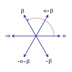
\begin{align*} [T_3, E_{\pm \alpha^{(2)}}] =\amp \pm \frac{1}{2} E_{\pm \alpha^{(2)}}, \qquad [T_8, E_{\pm \alpha^{(2)}}] = \pm \frac{\sqrt{3}}{2} E_{\pm \alpha^{(2)}},\\ [T_3, E_{\pm \alpha^{(3)}}] =\amp \pm \frac{1}{2} E_{\pm \alpha^{(3)}}, \qquad [T_8, E_{\pm \alpha^{(3)}}] = \mp \frac{\sqrt{3}}{2} E_{\pm \alpha^{(3)}}. \end{align*}

Thus the remaining four roots are $\pm (\frac{1}{2}, \frac{\sqrt{3}}{2})$ and $\pm (\frac{1}{2}, - \frac{\sqrt{3}}{2})\text{.}$ The resulting root system is shown in Figure 5.9.12.

Figure 5.9.12. The root system for $\mathfrak{su}(3)$ (taken from wikipedia).

🔗

But our goal here is not to construct representations, but to classify simple Lie algebras. It turns out that the roots are key for this as well. Indeed, the roots tell us not only something about the adjoint representation, but in fact they can be used to reconstruct the whole algebra itself. This is perhaps expected, since the adjoint representation is defined in terms of the structure constants, and hence should package the information content of the Lie algebra itself.

🔗

To see how this goes we need a few more definitions.

🔗

Definition 5.9.13. Positive and simple root.

A positive weight is a weight of a representation such that the first non-zero component is positive. A positive root is a positive weight for the adjoint representation. A simple root is a positive root that cannot be written as a linear combination of other positive roots with all coefficients being positive.

🔗

One can show that knowing the simple roots is in fact sufficient to determine all roots of a Lie algebra, because of the symmetries of a root system. The simple roots in fact form a basis for

$\mathbb{R}^m\text{,}$ so, in particular, there are

$m$ simple roots, where

$m$ is the rank of the Lie algebra.

🔗

Example 5.9.14. Simple roots for $\mathfrak{su}(3)$ .

In Example 5.9.11 we determined that the roots of $\mathfrak{su}(3)$ are $\pm (1,0)\text{,}$ $\pm (\frac{1}{2}, \frac{\sqrt{3}}{2})$ and $\pm (\frac{1}{2}, - \frac{\sqrt{3}}{2})\text{.}$ The positive roots are then $(1,0)\text{,}$ $(\frac{1}{2}, \frac{\sqrt{3}}{2})$ and $(\frac{1}{2}, - \frac{\sqrt{3}}{2})\text{.}$ Since

\begin{equation*} (1,0) = (\frac{1}{2}, \frac{\sqrt{3}}{2}) + (\frac{1}{2}, - \frac{\sqrt{3}}{2}), \end{equation*}

we see that $(1,0)$ is not a simple root. The other two positive roots, $(\frac{1}{2}, \pm \frac{\sqrt{3}}{2})\text{,}$ are the simple roots of $\mathfrak{su}(3)\text{.}$

🔗

Subsection 5.9.3 Root systems

🔗

The discussion of the preceding section shows that to a Lie algebra

$\mathfrak{g}\text{,}$ we can associate a bunch of roots living in weight space

$\mathbb{R}^m$ by looking at the eigenvalues of the adjoint representation. These roots form what is called a root system. It turns out that root systems are very constrained. Random bunch of vectors in

$\mathbb{R}^m$ certainly do not form root systems for some Lie algebra. It turns out that root systems can be defined abstractly, independently of Lie algebras, which we now do. In fact, we note here that root systems appear in many different contexts in mathematics, not just in the context of Lie theory.

🔗

Definition 5.9.15. Root system.

A root system $\Phi$ in $\mathbb{R}^m$ is a finite number of vectors (roots) in $\mathbb{R}^m$ such that:

The roots span $\mathbb{R}^m\text{.}$
For any root $\alpha \in \Phi\text{,}$ the only scalar multiple of $\alpha$ that is also in $\Phi$ is $- \alpha\text{.}$
For every $\alpha \in \Phi\text{,}$ $\Phi$ is closed under reflections through the hyperplane perpendicular to $\alpha\text{.}$ This can be rephrased as the condition that for any two $\alpha,\beta \in \Phi,$ we must have that
$\begin{equation*} \sigma_\alpha(\beta) = \beta - 2 \frac{\alpha \cdot \beta}{\alpha \cdot \alpha} \in \Phi. \end{equation*}$
For any two $\alpha,\beta \in \Phi,$
$\begin{equation*} 2 \frac{\alpha \cdot \beta}{\alpha \cdot \alpha} \in \mathbb{Z}. \end{equation*}$

🔗

Note that one can construct root systems by “putting together” smaller root systems. Two roots systems can be combined into a bigger one by considering the spaces

$\mathbb{R}^{m_1}$ and

$\mathbb{R}^{m_2}$ as mutually orthogonal subspaces of a bigger space

$\mathbb{R}^{m_1 + m_2}\text{.}$ Then the two roots systems form a bigger root system in

$\mathbb{R}^{m_1+m_2}\text{.}$ We say that root systems that cannot be obtained in this way are irreducible. In other words, a root system

$\Phi$ is irreducible if it cannot be partitioned into two roots systems

$\Phi = \Phi_1 \cup \Phi_2$ such that

$\alpha \cdot \beta = 0$ for all

$\alpha \in \Phi_1$ and

$\beta \in \Phi_2\text{.}$

🔗

The crucial result in our context is that there is a one-to-one correspondence between simple Lie algebras and irreducible roots systems (up to isomorphisms). This is absolutely key. We have already seen how, given a Lie algebra

$\mathfrak{g}\text{,}$ we can calculate its roots, which are the weights of its adjoint representation. Then one can show that for any simple Lie algebra, these roots form an irreducible root system, according to the definition above. So we know that we can assign a unique irreducible root system to a simple Lie algebra.

🔗

What needs to be shown is the reverse direction. First, we must show that starting with an irreducible root system, we can assign at most one associated simple Lie algebra. In other words, two non-isomorphic simple Lie algebras cannot share the same irreducible root system. This is not so trivial, but intuitively, it is expected, since two non-isomorphic simple Lie algebras cannot have the same structure constants, and hence cannot have the same roots. Second, we must show that to any irreducible root system one can assign at least one simple Lie algebra. In other words, that any irreducible root system arises as the root system of a simple Lie algebra. As we will see, this is clear for the four infinite families of irreducible root systems, since those arise as root systems of basic matrix Lie groups. But it is not so obvious to prove for the five exceptional root systems.

🔗

Subsection 5.9.4 Classification of simple Lie algebras

🔗

The fact that simple Lie algebras are in one-to-one correspondence with irreducible root systems (up to isomorphisms) imply that to classify simple Lie algebras, we only need to classify irreducible root systems, which is a nice combinatorial problem. Root systems are in fact nicely encapsulated into so-called Dynkin diagrams.

🔗

We construct the Dynkin diagram associated to a root system

$\Phi$ as follows. We assign a node to each of the simple roots. Then we draw edges between nodes according to the angle between the roots. The definition of a root system implies that the only possible angles between root vectors are

$\pi/2\text{,}$

$2 \pi/3\text{,}$

$3 \pi/4$ and

$5 \pi /6\text{.}$ We draw and edge between nodes as follows:

No edge if the root vectors are perpendicular ( $\pi/2$ );
A single edge if the angle between the root vectors is $2 \pi /3\text{;}$
A double edge if the angle between the root vectors is $3 \pi /4\text{;}$
A triple edge if the angle between the root vectors is $5 \pi /6\text{.}$

🔗

Moreover, in the last two cases, one can show that the two root vectors cannot have equal length. Thus we draw an arrow pointing towards the shorter vector.

🔗

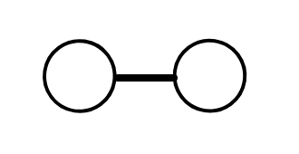
Example 5.9.16. Dynkin diagram for $\mathfrak{su}(3)$ .

Going back to $\mathfrak{su}(3)\text{,}$ we found that the two simple roots are given by $(\frac{1}{2}, \pm \frac{\sqrt{3}}{2})\text{.}$ So the Dynkin diagram will have two nodes. The angle between the two simple roots is $2 \pi /3\text{,}$ and hence the two nodes are connected by a single edge. The Dynkin diagram of $\mathfrak{su}(3)$ is shown in Figure 5.9.17.

Figure 5.9.17. The Dynkin diagram for $\mathfrak{su}(3)\text{.}$

🔗

Using Dynkin diagrams, one can classify all possible irreducible root systems, and hence all simple Lie algebra (up to isomorphisms). The classification is shown in Figure 5.9.18. It turns out that there are four infinite families, usually denoted by

$A_n, B_n, C_n$ and

$D_n\text{,}$ and five exceptional cases, denoted by

$G_2\text{,}$

$F_4\text{,}$

$E_6\text{,}$

$E_7$ and

$E_8\text{.}$

🔗
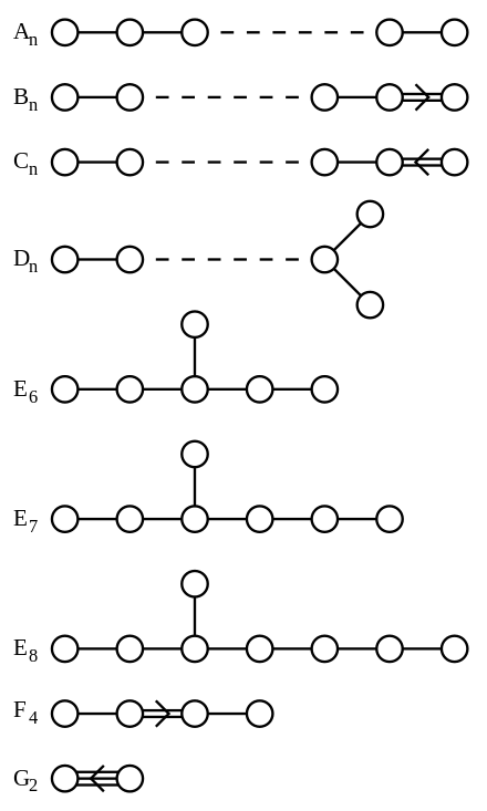
Figure 5.9.18. Classification of irreducible root systems in terms of Dynkin diagrams (taken from wikipedia).

🔗

The infinite families correspond to the root systems of well-known simple Lie algebras. We have that

$A_n \cong \mathfrak{su}(n+1)\text{,}$

$B_n \cong \mathfrak{so}(2n+1)\text{,}$

$C_n \cong \mathfrak{sp}(2n)\text{,}$ and

$D_n \cong \mathfrak{so}(2n)\text{.}$ The only family that we have not studied in this class is

$C_n \cong \mathfrak{sp}(2n)\text{,}$ which corresponds to the Lie algebra associated to

$2n \times 2n$ symplectic matrices.

🔗

The five exceptional root systems also correspond to simple Lie algebras, but those are not realized in terms of matrices with simple properties (such as orthogonal, unitary, symplectic, etc.) But these exceptional Lie algebras are common in physics: for instance, in one flavour of string theory (so-called “heterotic string theory”), the starting gauge group of the theory is

$E_8 \times E_8\text{,}$ where

$E_8$ is the Lie group whose Lie algebra has root system given by the

$E_8$ exceptional case.

🔗

Remark 5.9.19.

Looking at Figure 5.9.18, we see that the infinite families $A_n$ and $D_n\text{,}$ as well as the exceptional cases $E_6, E_7, E_8$ are special because they only have single edges. We call such diagrams simply laced. Those Dynkin diagrams arise often in many different contexts in mathematics. Whenever these diagrams arise, we refer to their classification in mathematics as an ADE classification.