Tangible Computing - 21. Dynamic Programming

Tangible Computing

21. Dynamic Programming

21.1 Recursive decomposition of problems

When we discussed sorting, we drew the standard diagram for merge sort showing how the sorting problem for n elements was decomposed into n/2 small pair-sorting problems and then the results combined.

The key thing about these divide and conquer problems is that the problem is decomposed into independent subproblems. That is, the subproblems typically do not share any details in common.

Divide and conquer algorithms typically break the problem size in half at each step, and thus have complexity that looks like O(n long n).

Now, contrast this the recursive computation of the Fibonacci sequence, which is defined as follows

code/DynamicProg/fib.py

# Fibonacci example

import sys

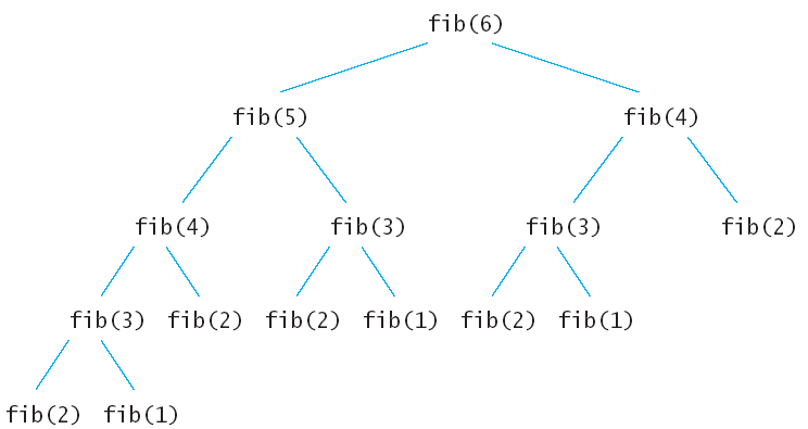
def fib(n):

if n == 0: return 1

if n == 1: return 1

return fib(n-1) + fib(n-2)

# fetch n from the command line args

if len(sys.argv) > 1:

k = int(sys.argv[1])

else:

k = 10

f = fib(k)

print("Fib ", k, " is ", f)

The recursive decomposition three for computing Fib(6) looks like this.

If we instrument the code, we see that computing Fib this way results in an exponential size recursion tree!

code/DynamicProg/fib-instrument.py

# Fibonacci example

import sys

def fib(n):

global call_count

call_count += 1

if n == 0: return 1

if n == 1: return 1

return fib(n-1) + fib(n-2)

if len(sys.argv) > 1:

k = int(sys.argv[1])

else:

k = 10

call_count = 0

f = fib(k)

print("Fib ", k, " is ", f, " work ", call_count);

But, many of the subproblems in this tree are identical. In fact, there for Fib(n) there are only n+1 unique subproblems. If we keep a record of the subproblems that we solve, using a technique called memoization (which is a form of caching) then we can compute Fib using only a linear number of sub-problems.

code/DynamicProg/fib-memo.py

# Fibonacci example, with memoization

import sys

# Fibonacci is defined as: fib(n) = fib(n-1) + f(n-2), where

# fib(0) = 1, fib(1) = 1 (or any other acceptable initial conditions)

# when we compute fib, there is considerable overlap between the recursive

# sub-problems. So this is not a divide and conquer where the sub-problems

# are independent. So it makes sense to keep track of prior solutions of

# sub-problems.

# Alternatively, we can do the computation forward, since we can write

# fib(n+2) = fib(n+1) + fib(n)

# and in this case need only store the "frontier" of the last 2 values.

# remember previously computed values of fib, including the base cases

fib_at= { 0: 1, 1: 1 }

def fib(n):

global call_count

global fib_at

# have we computed fib(n) already?

if n in fib_at: return fib_at[n]

# no, so count this work

call_count += 1

f = fib(n-1) + fib(n-2)

fib_at[n] = f

return f

if len(sys.argv) > 1:

k = int(sys.argv[1])

else:

k = 10

call_count = 0

f = fib(k)

print("Fib ", k, " is ", f, " work ", call_count);

Note: of course, no one computes Fib recursively, since you can compute it directly by working up from the initial cases.

In general, dynamic programming should be considered in a situation with these characteristics:

An instance of the problem can be divided into two or more smaller sub-problems.
The number of distinct sub-problem instances that would be considered in solving the problem is significantly smaller than the total number of sub-problems the probelm is decomposed into.

21.2 Floyd-Warshall All-Pairs Min-Cost Paths

A more interesting example of dynamic programming is the Floyd-Warshall algorithm to compute the set of minimum cost paths between all pairs of vertices in a graph.

The problem of finding a minimum cost path between two vertices, say with DIjkstra's Algorithm, you see that many smaller minimum cost path problems are being solved. In fact, the minimum cost paths between two different pairs of vertices might have many edges in common. This suggests that we can decompose the minimum cost path problem in a number of smaller minimum cost path problems, and then exploit the large number of common sub-problems.

Suppose there are n vertices in the graph. The n x n adjacency matrix A has entries as follows:

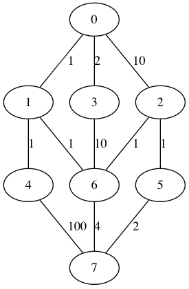
A[i, i] = 0 for 0 <= i < n
A[i, j] = the cost of the edge from i to j

All entries are non-negative (>= 0), and and entry is infinity if there is no edge.

Here is a sample adjacency matrix code/DynamicProg/adj.txt

0 1 10 2 N N N N

1 0 N N 1 N N N

10 N 0 N N 1 2 N

2 N N 0 N N 10 N

N 1 N N 0 N 1 100

N N 1 N N 0 N 2

N N 2 10 1 N 0 4

N N N N 100 2 4 0

corresponding to this undirected graph.

All of the following discussion works for both undirected and directed graphs.

Next, we will consider decomposing the problem in terms of the best solutions (i.e. minimum cost paths) we can find, given the constraint that they have at most k edges in them. We define a sequence of matrices Cost_k, k = 0, 1, 2, ... where the entry in the matrix is:

Cost_k[i, j] = minimum cost of a path of k or less edges from i to j

Then we showed how we can extend a solution for k to a solution with one more edge by observing that the minimum cost path of length k+1 or less from vertex s to vertex d is either one of length k or less, or is one of length k+1 that is found by exploring one more edge along a minimum cost path of length k. That is,

Cost_(k+1)[s, d] = min over i { Cost_k[s, i] + A[i, d] }

where we observe that A[i,i] = 0 so that paths of length k or less are also considered.

This then resulted in an interesting observation that we can formulate the minimum cost path problem in terms of a matrix multiplication problem

Cost_(k+1) = Cost_k x A = A^k

where the 'x' operation is the (min, +) vector dot product. That is, do a pairwise add of the elements and then select the min. Of we can compute Cost_n then we have the min cost of a path between any pair of vertices.

A single matrix multiplication is O(n^3), because it consists of n^2 elements, each of which takes O(n) to compute. So the complexity of computing Cost_n is the complexity of computing A^n, which is O(n^4).

But, if we want to compute A^n, we can use a divide a conquer approach of doign O(lon n) squarings of the matrix. Thus computing the min cost of a path for all pairs of source and destination vertices is O(n^3 log n).

The only problem with this is that we do not have an actual path for each pair. Suppose that you have the adjacency matrix A and all of the Cost_k matrices for k = 1, ..., n.

A path is simply a list of pairs, like

[(0, 1), (1, 4), (4, 3)]

which is a path of 3 edges from 0 to 3.

Let Path_k[i, j] be a list of k or less edges that give a min cost path from from i to j with cost Cost_k[i, j]. That is, Path_k gives the paths corresponding to the Cost_k matrix.

Exercise Part 1: Write the equations that show how the computation of Path_(k+1) can be reduced to the computation (or look up in this case) of Cost_k and Cost_(k+1). You also have A at your disposal, and of course any Path_k that you have computed.

Hint: Here is the easy part of the reduction.

Path_1[i, i] = [ ]
Path_1[i, j] = [ (i, j) ] if A[i,j] != Infinity
Path_1[i, j] = None if A[i,j] == Infinity
Path_(k+1)[i, j] = Path_k[i, j] if Cost_(k+1)[i, j] = Cost_k[i, j]

You need to define Path_(k+1) for the remaining case.

Exercise Part 2: What is the complexity of your reduction, assuming that the cost matrix lookups are O(1)?

21. Dynamic Programming
Tangible Computing / Version 3.20 2013-03-25