Statistical Analysis
In addition to data management, the foundation of this
project is the appropriate application of a variety of multivariate statistical
procedures. Ecological niche modelling, by definition, incorporates a large
number of environmental variables. While this is critical for producing accurate
niche models, it is desirable also to reduce redundant or highly correlated
variables in order to simplify the models and analysis. Furthermore, applying
ecosystem classifications to modern and paleoclimate data requires a
sophisticated data analysis procedure. Both of these tasks, variable
simplification and classification, can be accomplished through specific
multivariate statistical techniques. While there are a variety of statistical
packages available, the analyses performed on this project were conducted with SAS
v.9.1 for Windows.
It should be noted that, for this project, all data processing and modelling was completed using ecosystem variant/seed-zone classifications. However, all maps and outputs are shown in ecosystem zones. The variant classifications are simply too complex and the resolution too fine to display at any reasonable scale. For more information on the ecosystem classification hierarchy, please see 'Data and Data Management'. For a colour legend of ecosystem zone classifications (matches the zone classification images on this page), please click here (spawns a new window - hold CTL key and click to disable your pop-up blocker if necessary).
1) Principal Component Analysis (PCA) (Top)
Principal component analysis is a rotational technique
designed to isolate 'key' variables of a multivariate data set which describe
most of the variance in the entire data set. The idea is to find correlated data
variables and simplify these into specific variable that account for most of the
difference (variation) in the data. Ideally, a large data set contains many
correlated variables that may be explained by a few key variable, thus allowing
for the analysis of a few variables rather than the entire set (Manly 2005).
.PNG)
(Click for larger image)
|
The eigenvectors (loadings) from the PCA show the correlation of a few variables in the first two principal components. It would appear that Prin1 tends to favour the moisture-related variables as well as a measure of continentality. Prin2 seems to better represent the temperature variables including growing degree days. Interestingly, Prin3 appears to be a hybrid of sorts of the first two components--mixing variables of temperature, moisture, and continentality. I focused mainly on the first two components as I felt they most accurately represented the important climatic variables for vegetation. Also, I don't feel that focusing on Prin3 adds any information to the analysis.
Unfortunately, there does not appear to be any 'key' variables that account for the majority of the variance in the data set. This is made evident by summing the variance explained for the first few principal components. The sum of the eigenvectors for each variable values indicates the variance explained by the specific principal component. This can be expressed as a percentage by dividing the sum by the number of variables:
- Prin1: eigenvector total = 3.45, variance explained = 24.6%
- Prin2: eigenvector total = 3.21, variance explained = 22.9%
While it is advantageous to have few variables with high loadings (not seen in this case), I believe the split seen in this principal component analysis effectively splits the variables into moisture and temperature--a split that will prove useful in future analysis (see plot below).
On a side note, the 7th principal component (Prin7) in this analysis is very interesting in that it accounts for roughly the same variance explained as either of the first two principal components. However, it seems to represent winter conditions more than anything, showing high loadings for winter precipitation (negatively), extreme cold temperature, and degree days below 0C. Admittedly, this arrangement of correlations was overlooked in my original analysis. I feel it could be insightful to investigate this variable arrangement further for potential vegetation responses. See 'Future Directions' for more thoughts on this.
|
|
.PNG)
(Click for larger image)
|
Plotting the first two principal components
shows a good clustering of ecosystem sub-zones. As mentioned previously, the first two principal components show a reasonable and convenient split into moisture variables (Prin1, on the y-axis) and temperature variables (Prin2, on the x-axis).
While there are still
ecosystem classifications that show some scatter, this tend to be towards
the edges of the plot--particularly towards the left extreme. This would indicate that there are 'outlier' data
points of extreme and unique climatic conditions. This is to be expected, as it represents the alpine classification areas. In these areas, the low temperature values (weighted heavily in Prin2) drive these data points to the left side of the plot.
A quick inspection of many of the point classifications also provides a quick and intuitive check on the nature of the principal component analysis. If we interpret Prin1 as moisture variables (y-axis) and Prin2 as temperature variables (x-axis), we see expected ecosystem classifications in reasonable locations throughout the plot:
- ATnc1 (glacial ice) - appears in the extreme low temperature and high moisture areas
- BGxh (bunchgrass), PPxh (ponderosa pine), DMG (dry mixedgrass) - appears in the high temperature and low moisture areas
- CWHvm (coastal western hemlock) - appears in the high temperature and high moisture areas
- BWBSd (boreal white & black spruce) - appears in the moderate to low temperature and low moisture areas
Note: the colours on this plot DO NOT correspond to the colours in the provided ecosystem zone legend. For a comprehensive explanation of the ecosystem classification codes (MS Excel format), please click here. (Both links spawn a new window - hold CTL key and click to override your pop-up blocker.)
|
2) Discriminant Function Analysis (DISCRIM) (Top)
Discriminant analysis (DISCRIM), like PCA, is a rotational
technique for applying classifications or defining groups of individuals from a set of multivariate data, based on a defined set of variables. From a set of known variables with associated classifications, the DISCRIM procedure essentially produces vectors for each classification. Then, it examines the unclassified sets of variables and calculates to which existing classification the new data point most closely matches (by measuring the Mahalanobis distance to the known group centre). Because the known classified variables are also reclassified, it is possible to assess the accuracy of the classification method based on how many known data points were classified correctly (Manly 2005). The DISCRIM procedure is similar in function and process to a cluster analysis, but uses established classifications to classify the novel data rather than building groups "from scratch" based on groupings of data points.
The DISCRIM procedure requires a set of variables paired with known classifications (a calibration data set). I began with the baseline data for Alberta and British Columbia. This is a complete climate data set with known ecosystem classifications for each data point. Choosing the appropriate variables to consider in the discriminant analysis is key to the accuracy and generalizability of the classification procedure. The choice of included variables could be based on the outputs of my principal component analysis. Any 'key' variables identified in that procedure could be used to simplify the DISCRIM procedure through a reduction of input variables. However, due to low levels of variance explained in the PCA, I was hesitant to drop too many climate variables in this classification.
An advantage of discriminant analysis, as mentioned previously, is the ability to assess the classifications of the known data points. In the case of this data set, I found the greatest classification accuracy when all the climatic variables were included.

(Click for larger image) |
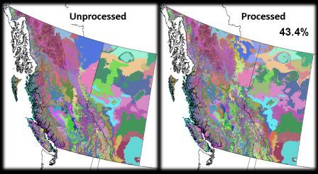
The DISCRIM procedure run on the ecosystem variant classifications with all the climate variables included produced a classification accuracy of 43.4%.
Note: the colours on this plot DO NOT correspond to the colours in the provided ecosystem zone legend. The actual ecosystem descriptions in this case are not as important as the distribution of the classes.
|

(Click for larger image)
|
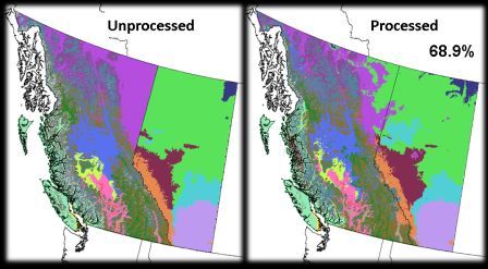
When the results of this discriminant analysis are considered at the zone level, the classification accuracy increases to 68.9%.
It should be noted that these classification accuracies may be somewhat skewed towards misclassification. Because I have combined ecosystem classifications from both Alberta and British Columbia, there are overlapping classifications--ecosystems that are essentially identical in Alberta and B.C., but are assigned different classifications in either province. An example of this can be seen easily along the northern border of the two provinces. In B.C., the BWBS (Boreal White & Black Spruce) zone is essentially identical in species and structure as the Alberta BF (Boreal Forest) zone. However, any overlap across the political boundary between the two provinces will be interpreted as a misclassification.
This is not only the case along the borders, however. Even within the interior of both provinces, there may be areas that suffer from this problem of redundant classifications. Essentially, neither classification (Alberta or B.C. equivalent) is incorrect despite being interpreted as such by the accuracy calculation. For more information on resolving this redundant classification issue, see 'Future Directions'.
|
Using this baseline data as a calibration for the discriminant analysis procedure, it is possible to apply the same classification technique to the entire western North America study area--for both the current period and for the paleoclimate data. Because the current data and paleoclimate data variables as in the baseline data, it is possible to use those same variables to assign the paleoclimate data to the same ecosystem classifications. Simply put, the paleoclimate data will be assigned as ecosystem classification just as if it were part of the original data set. The outputs of this analysis can be found on the 'Results & Discussion' page.
<<<< Back to Data & Data Management | Top of this page | Continue on to Results & Discussion >>>>
References:
Manly, B. F. J.
(2005). Multivariate Statistical Methods:
A Primer. 3rd Ed. Chapman & Hall / CRC Press, Boca Raton.
© 2007 - David Roberts, University of
Alberta

