When electrons scatter they can emit real photons. This process is called bremsstrahlung because it involves an acceleration or deceleration (in German ``bremson'') of the projectile. This bremsstrahlung or deceleration radiation with the emission of a single photon is a well-defined process only within certain limits: the simultaneous emission of very soft photons - too soft to be observed within the accuracy of the energy determination of the incident and outgoing electron - can never be excluded. In fact, this radiation is always present, even in so-called elastic scattering. Therefore, it will be impossible to make a clean physical distinction between bremsstrahlung and radiationless scattering when the emitted photon is very soft. We shall restrict ourselves, therefore to the emission of one not-too-soft photon.
Consider the emission of radiation of a charged particle (electron) in
the presence of an external field.
The four-vector potential of a photon with momentum
![]() and polarization
and polarization
![]() is written in Heaviside-Lorentz system
of units as the plane wave
is written in Heaviside-Lorentz system
of units as the plane wave
| (7.180) |
For simplicity we return to the static approximation and replace the
photon by a static Coulomb field and calcualte ![]() to lowest
non-vanishing order in
to lowest
non-vanishing order in ![]() .
There can be no first-order emission of radiation by a free electron
in the absence of the external filled.
This is kinematically forbidden, since it is impossible to conserve
energy and momentum:
.
There can be no first-order emission of radiation by a free electron
in the absence of the external filled.
This is kinematically forbidden, since it is impossible to conserve
energy and momentum:
![]() .
.
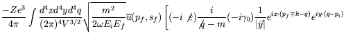
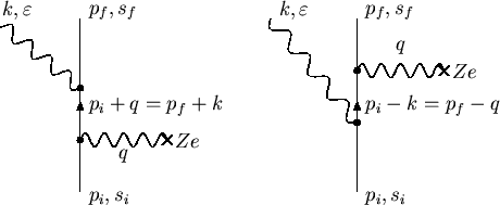
The Feynman diagrams (figure 7.5) for this process correspond to a second-order process with one vertex for the interaction of the electron with the Coulomb field and one for the emission of the bremsstrahlung quantum.
The second-order ![]() -matrix element is
-matrix element is
| (7.181) |
where
![]() ,
and the two terms correspond to the two orderings of the vertices.
,
and the two terms correspond to the two orderings of the vertices.
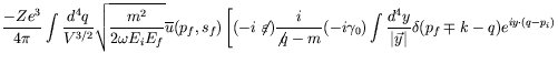
It is convenient to transform to momentum space by Fourier-expanding all factors and carrying out the coordinate integrations.
 |
|||
 |
|||
 |
|||
 |
|||
| (7.182) |
where ![]() and we have taken the
and we have taken the ![]() solution only.
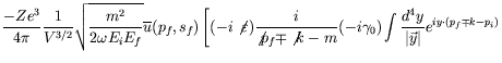
There is an additional contribution coming from the first term of the
photon potential for which the energy
solution only.
There is an additional contribution coming from the first term of the
photon potential for which the energy ![]() -function is
-function is
![]() .
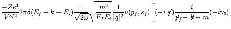
This term describes absorption of energy in the scattering process and
does not contribute to the process of interest here, in which the
incident electron gives up energy to the radiation field and emerges
with
.
This term describes absorption of energy in the scattering process and
does not contribute to the process of interest here, in which the
incident electron gives up energy to the radiation field and emerges
with ![]() .
.
We notice the factor
![]() appears at the vertex where a free
photon of polarization
appears at the vertex where a free
photon of polarization
![]() is emitted, and
is emitted, and
![]() appears as the normalization factor for a photon wave function
appears as the normalization factor for a photon wave function
We limit our derivation to
![]() , or to the emission of a
very soft photon.
The more general result is known as the Bethe-Heitler formula.
In the limit of
, or to the emission of a
very soft photon.
The more general result is known as the Bethe-Heitler formula.
In the limit of
![]() the factor within brackets can be
approximated as
the factor within brackets can be
approximated as
Proceeding to the cross-section, we square ![]() , divide by the
flux
, divide by the
flux
![]() and by
and by ![]() to form a rate,
and sum over final states
to form a rate,
and sum over final states
![]() in the observed
interval of phase space.
We obtain
in the observed
interval of phase space.
We obtain
| (7.184) |
Identifying terms with the elastic scattering cross-section (equation 7.44) we find
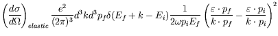 |
|||
 |
(7.185) |
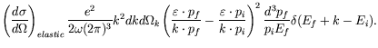
Using
| (7.186) |
we have
| (7.187) |
Since
![]() , we can take
, we can take
![]() .
Using
.
Using
| (7.188) |
we have
| (7.189) |
This is the cross-section for the electron to be observed in a solid
angle ![]() and for a photon of polarization
and for a photon of polarization ![]() to
emerge with
to
emerge with ![]() in the interval
in the interval ![]() .
.
The result is more general than one might expect.
It has been shown that in the limit
![]() the amplitude for
any process leading to photon emission can be factorized according to
the amplitude for
any process leading to photon emission can be factorized according to
| (7.190) |
where ![]() is the amplitude for the same process without photon emission.
This result is true for any kind of process, irrespective of the spin or
internal structure of the charged particle.
is the amplitude for the same process without photon emission.
This result is true for any kind of process, irrespective of the spin or
internal structure of the charged particle.
We notice that the photon energy spectrum behaves as ![]() and
therefore for the probability to emit a zero-energy photon is
infinite.
This is the ``infrared catastrophe''.
For a consistent comparison with experiment we must include both
elastic and inelastic cross-sections calculated to the same order in
and
therefore for the probability to emit a zero-energy photon is
infinite.
This is the ``infrared catastrophe''.
For a consistent comparison with experiment we must include both
elastic and inelastic cross-sections calculated to the same order in
![]() .
Since the bremsstrahlung contribution is of order
.
Since the bremsstrahlung contribution is of order ![]() relative to
the elastic scattering, we must also include radiative corrections to
relative to
the elastic scattering, we must also include radiative corrections to
![]() to the same order
to the same order ![]() .
These correspond to second-order scattering of the electron in the
Coulomb field plus we must take into account the interaction of the
electron with itself via the radiation field (figure 7.6).
The amplitude coming from these later processes contain a divergent
term which precisely cancels the divergence at
.
These correspond to second-order scattering of the electron in the
Coulomb field plus we must take into account the interaction of the
electron with itself via the radiation field (figure 7.6).
The amplitude coming from these later processes contain a divergent
term which precisely cancels the divergence at ![]() .
.
Before evaluating the matrix element, we look at how gauge invariance of
the electromagnetic field puts a condition on the electromagnetic
current in momentum space.
The interaction of any electromagnetic current, ![]() , with the
vector potential,
, with the
vector potential, ![]() , is given by
, is given by
| (7.191) |
The integral must be invariant under the gauge transformation
| (7.192) |
Integrating by parts this implies
| (7.193) |
Since ![]() is an arbitrary function this yields the condition of
current conservation
is an arbitrary function this yields the condition of
current conservation
| (7.194) |
which can be written in momentum space as
| (7.195) |
This property is shared also by quantum mechanical transitions currents.
Thus we can expect that the matrix element
![]() satisfies
satisfies
| (7.196) |
since ![]() is the transition current for bremsstrahlung up to a
numerical factor.
Using the matrix element in equation 7.183 this condition is
easily shown to be true.
is the transition current for bremsstrahlung up to a
numerical factor.
Using the matrix element in equation 7.183 this condition is
easily shown to be true.
We now turn to the evaluation of the summation over the photon polarizations. The quantity of interest is
Since this is a scalar, we can evaluate it in an arbitrary Lorentz
frame.
Orienting the coordinates such that
![]() , where
, where
![]() , since
, since ![]() .
We choose
.
We choose ![]() .
In this system
.
In this system ![]() is transverse and the two independent
transverse polarizations may be written as
is transverse and the two independent
transverse polarizations may be written as
| (7.198) | |||
| (7.199) |
Therefore
![]() and
and
![]() ,
,
![]() and
and
![]() .
.
Summing over polarizations we have
| (7.200) |
Invoking our condition of current conservation, we have
| (7.201) |
which implies
![]() .
Then we transform into a four dimensional scalar product by adding the
vanishing contributions
.
Then we transform into a four dimensional scalar product by adding the
vanishing contributions
| (7.202) |
Since this result is covariant, we compare it with equation 7.197 to write
| (7.203) |
The additional gauge terms need not be specified in detail.
They are proportional to ![]() and
and ![]() and thus do not contribute
to any observable quantity since our result will be multiplied with
conserved currents which satisfy
and thus do not contribute
to any observable quantity since our result will be multiplied with
conserved currents which satisfy ![]() .
Nevertheless these terms have to be present since a complete basis in
4-dimension space of Lorentz vectors has to contain 4 elements.
The contribution of longitudinal
.
Nevertheless these terms have to be present since a complete basis in
4-dimension space of Lorentz vectors has to contain 4 elements.
The contribution of longitudinal
![]() and scalar
and scalar
![]() photons to the completeness relation makes
their appearance on the right-hand side of our result.
They do not correspond to physical photons however.
We have thus proven the completeness relation of the polarization
vectors.
photons to the completeness relation makes
their appearance on the right-hand side of our result.
They do not correspond to physical photons however.
We have thus proven the completeness relation of the polarization
vectors.
We now apply this completeness relation to the bremsstrahlung cross-section. Notice
| (7.204) |
and thus
| (7.205) |
Integrating over all photons emission angles and energies in the
interval
![]() gives
gives
| (7.206) |
Writing
![]() we have
we have
To integrate the last two terms in equation 7.207 we use
| (7.208) |
To evaluate the first integral we use
| (7.209) |
to obtain
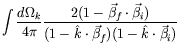 |
![$\displaystyle \int_0^1 dx \int\frac{d\Omega_f}{4\pi}
\frac{2(1-\vec{\beta}_f\cd...
...}_i)}
{[(1-\hat{k}\cdot\vec{\beta}_f)x +
(1-\vec{k}\cdot\vec{\beta}_i)(1-x)]^2}$](img3998.png) |
||
![$\displaystyle \int_0^1 dx\int\frac{d\Omega_f}{4\pi}
\frac{2(1-\vec{\beta}_f\cdot\vec{\beta}_i)}{[1-\hat{k}\cdot(\vec{\beta}_fx
+ \vec{\beta}_i(1-x))]^2} .$](img4000.png) |
(7.210) |
Using
| (7.211) |
we have
| (7.212) |
In the soft photon limit
![]() and
and
![]() .
Thus
.
Thus
In the non-relativistic limit (![]() ) the integral
(equation 7.213) becomes
) the integral
(equation 7.213) becomes
| (7.214) |
In the extreme relativistic limit
| (7.215) |
and
| (7.216) |
and the integral (equation 7.213) becomes
| (7.217) |
From a table of integrals
| (7.218) |
where ![]() .
Including the limits of integration we have
.
Including the limits of integration we have
| (7.219) |
For the case of ![]() and
and ![]()
| (7.220) |
where ![]() .
In our case
.
In our case ![]() and
and
![]() .
Thus
.
Thus
| (7.221) |
The integral (equation 7.213) now becomes
| (7.222) |
Therefore the soft bremsstrahlung cross-section is
| (7.223) |
![\begin{figure}\begin{center}
\begin{picture}(415,120)(-10,-10)
\SetWidth{0.75}
%...
...47)
\Text(105,50)[lc]{$Ze$}
\end{picture}}
\end{picture}\end{center}\end{figure}](img3933.png)
![$\displaystyle \left. -\frac{m^2}{E_f^2(1-\hat{k}\cdot\vec{\beta}_f)^2}
-\frac{m^2}{E_i^2(1-\hat{k}\cdot\vec{\beta}_i)^2} \right].$](img3987.png)