The Physics of Percolation
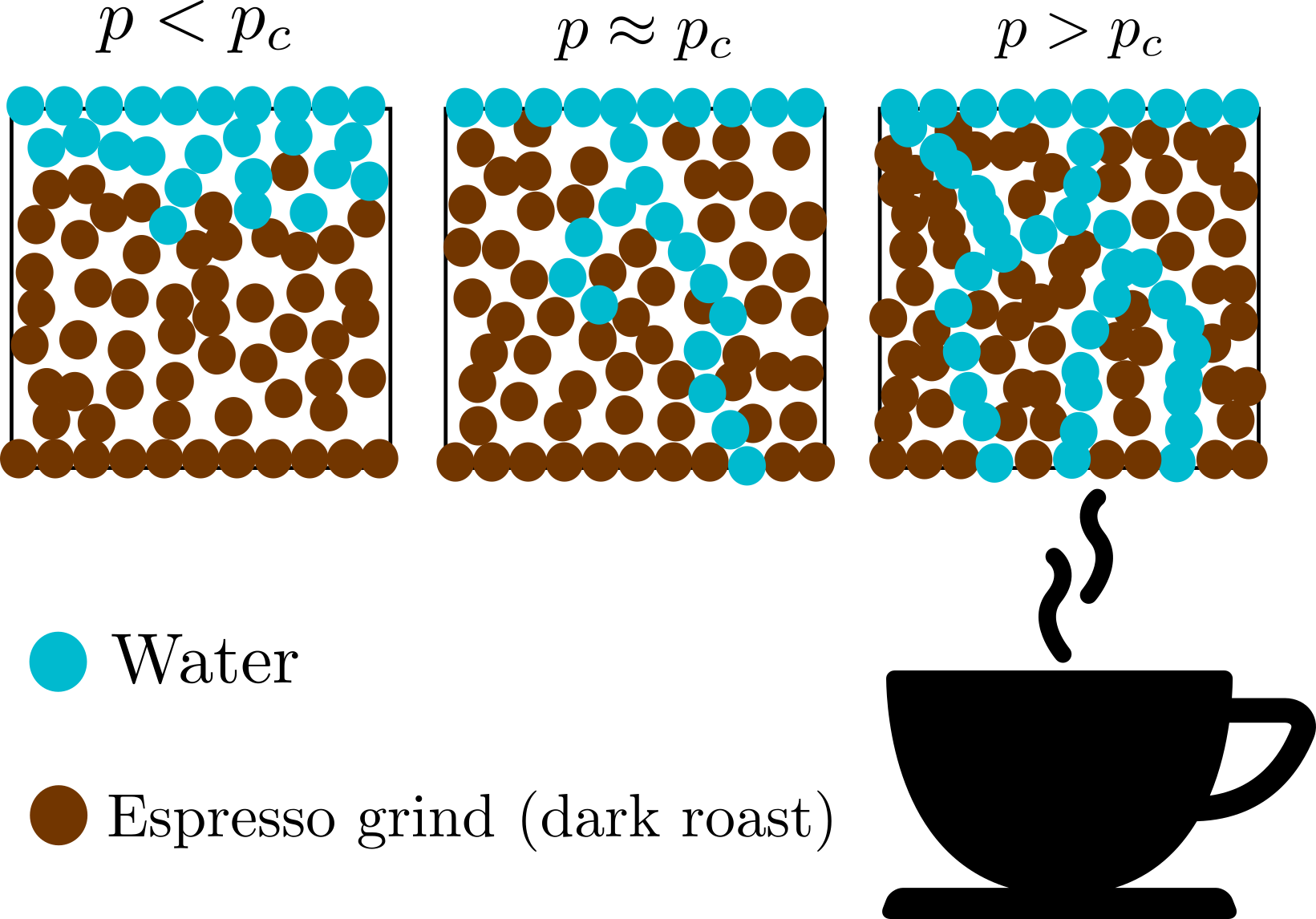
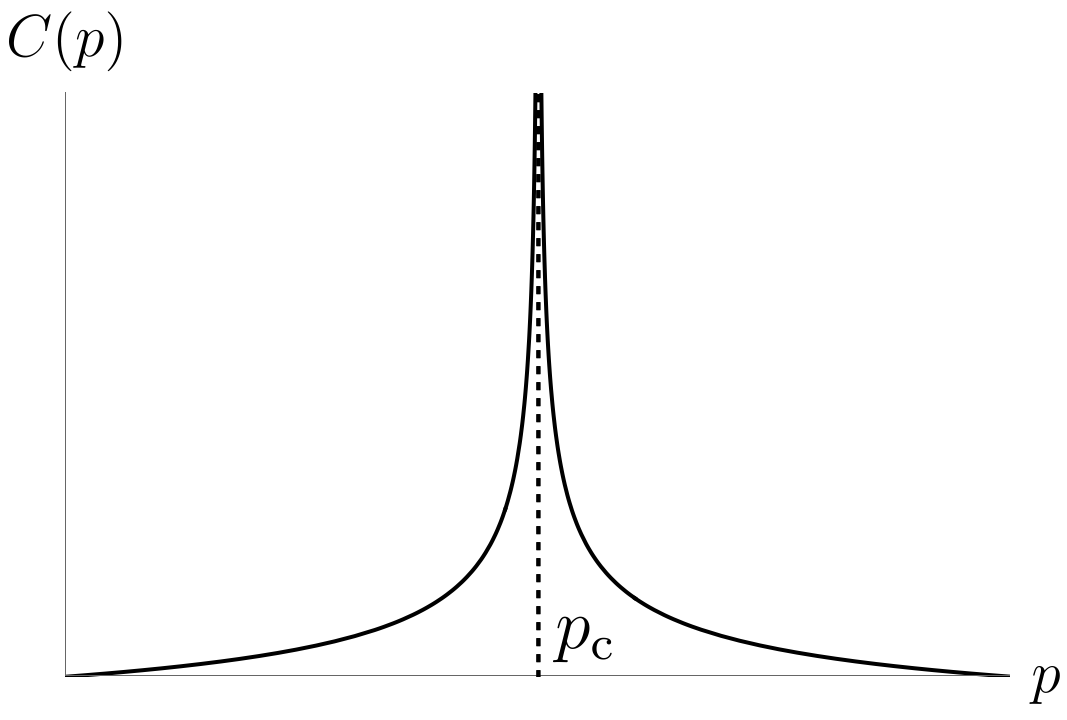
What does making an espresso, forest fires and Covid-19 have in common? Percolation theory! Percolation (from the latin word percolare) refers to the movement of fluids through porous materials, viz. water and espresso grinds. Percolation theory has found its place in a variety of fields like geology where its practical use is of great importance. However, it turns out that percolation has also found its place in the field of statistical physics where it embodies the incredibly deep concept of phase transitions and universality. To see the phase transition, let us think a bit more about how our water gets through the grinds. You might have noticed that if your espresso grinds are tamped too hard, then it’s near to impossible to extract coffee unlike the case of loosely packing it, in which you get a watery cup of coffee. Intuitively, it is the spacing or the fraction of air to coffee grinds that control the flow of water. If you imagine being able to control the fraction of air to espresso grinds during the process of extraction, then something magical happens as you vary this fraction from low to high. Small local pockets of air emerge randomly along the path of your coffee until these pockets start connecting to each other. When they do so, they pave the way for water to get (percolate) further through the grounds. These pockets of air slowly show up until you cross a certain threshold, after which water rushes through a path through the grinds and you suddenly get coffee! Like a phase transition in the case of a magnet, we may model this sudden onset of coffee as a phase transition with a certain critical threshold called the percolation threshold after which you are guaranteed coffee 1. For an illustration, see attached Fig. 1, and check out this fantastic animation (coffee flows from the left). Now, you may recognize the connection to forest fires where the “air” corresponds to trees that can catch on fire and the grinds correspond to the empty space between trees 2. Similarly, the connection exists in the spread of diseases where non-infected and infected play these roles respectively. In each of these examples, you may notice that the system is entirely different and indeed their percolation thresholds will be different too. Even in the case of using different grind sizes, the threshold changes because it depends on the finer details of the model. But there is something that does not change, something universal.
So what is universal about these systems? It turns out that if you study (plot) the amount of coffee with respect to the fraction of air right around this critical point, you find that the amount of coffee follows a power law, where the exponent is now aptly-named the critical exponent. What is bizarre is that this exponent is the same across different systems and only depends on a few features like the dimension and symmetries of the system. It is precisely in this sense that it is universal, and physicists have catalogued many different systems in their own so-called universality classes. The beauty of these universality classes is that if you know these exponents for one system, then you know all of them within the same class. This observation was first made by L. Kadanoff, a giant in statistical physics, who recognized that it is universality that enables us to study these simplified models for the real world out there, no matter how complex the finer details! Various mathematical models have been constructed to study percolation, the most simplest of which is Bernoulli percolation 3 that enables us to extract these exponents matching experiments.
Introduction
In this lab we are going to study the incredible physics of percolation. Percolation (from the latin word percolare) refers to the movement of fluids through porous materials, viz. water and espresso grinds. Percolation theory has found its place in a variety of fields like geology where its practical use is of great importance. However, it turns out that percolation has also found its place in the field of statistical physics where it embodies the incredibly deep concept of phase transitions and universality. Often, it is explained through making coffee–the grinds block the flow of coffee with small gaps randomly distributed due to mixing and the water (and hence coffee) flows through it. When the ratio of air to grinds is low (espresso dominated), the grinds are too thick and coffee cannot flow. However, when this ratio is high (gap dominated), coffee can easily flow. One can imagine varying this ratio from low to high until you hit a critical ratio of air to water $p_{\rm c}$ at which, you get coffee! For an illustration, see Fig. 1.
To emulate the physics of percolation in a lab setting, we’ll resort to using electrical measurements. We will replace air with metal beads and the espresso grinds as plastic beads of diameter 1/8” or 3.175 mm to do so. As you vary the fraction of metal beads to plastic beads, we will see the emergence of a critical threshold $p_{\rm c}$ in our Conductance and Capacitance measurements. The main goal of the lab is to measure the critical threshold $p_c$ that causes a sudden change in Conductance $G(p)$, Capacitance $C(p)$ and Admittance \(Y(p)= G(p)+ i \omega C(p)\) where $\omega$ is the fixed frequency of the current passing through the metal-plastic beads, followed by their corresponding power laws that follow them. We will conclude with your own open-ended experiment.
Main observables
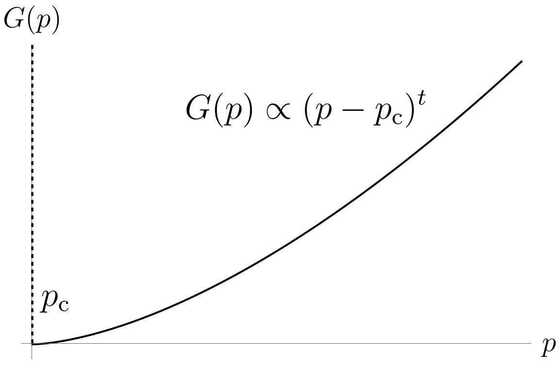
Around $p=p_c$, percolation theory predicts that around $p=p_c$, we should observe
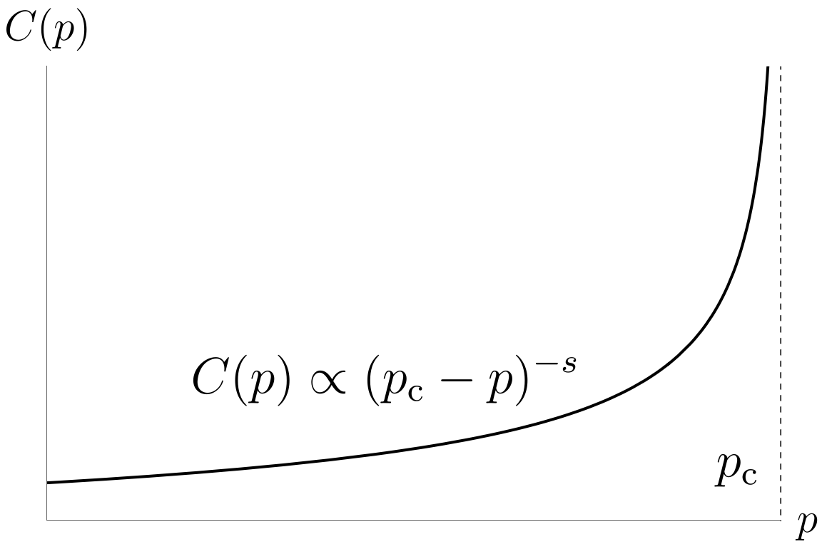
\(G(p) \propto (p-p_c)^t,\) \(C(p) \propto (p_c-p)^{-s},\)
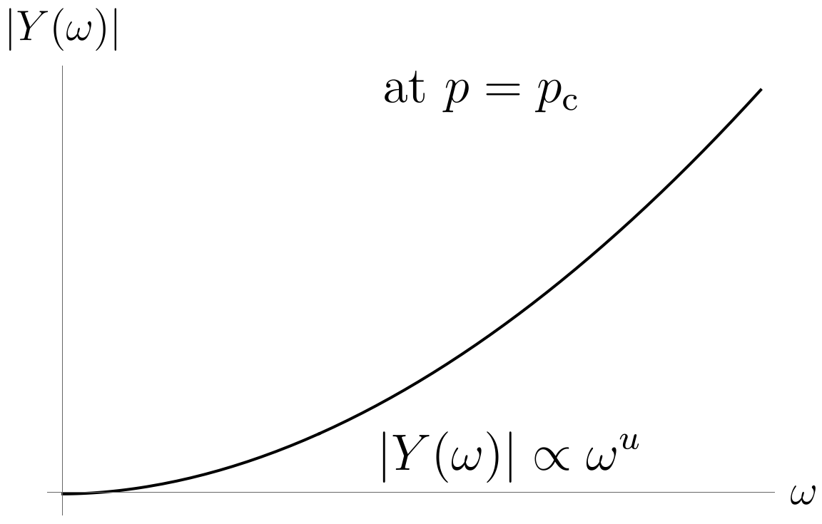
and at $p=p_c$ for changing frequencies,
\[|Y(\omega)|\propto \omega^u.\]At the end of the lab, we will measure the percolation threshold $p_c$, the conductance, capacitive and admittance exponents $t,s$ and $u$ respectively.
Over the next few weeks, we will grapple our experimental techniques to measure these quantities using our instruments.
Instruments
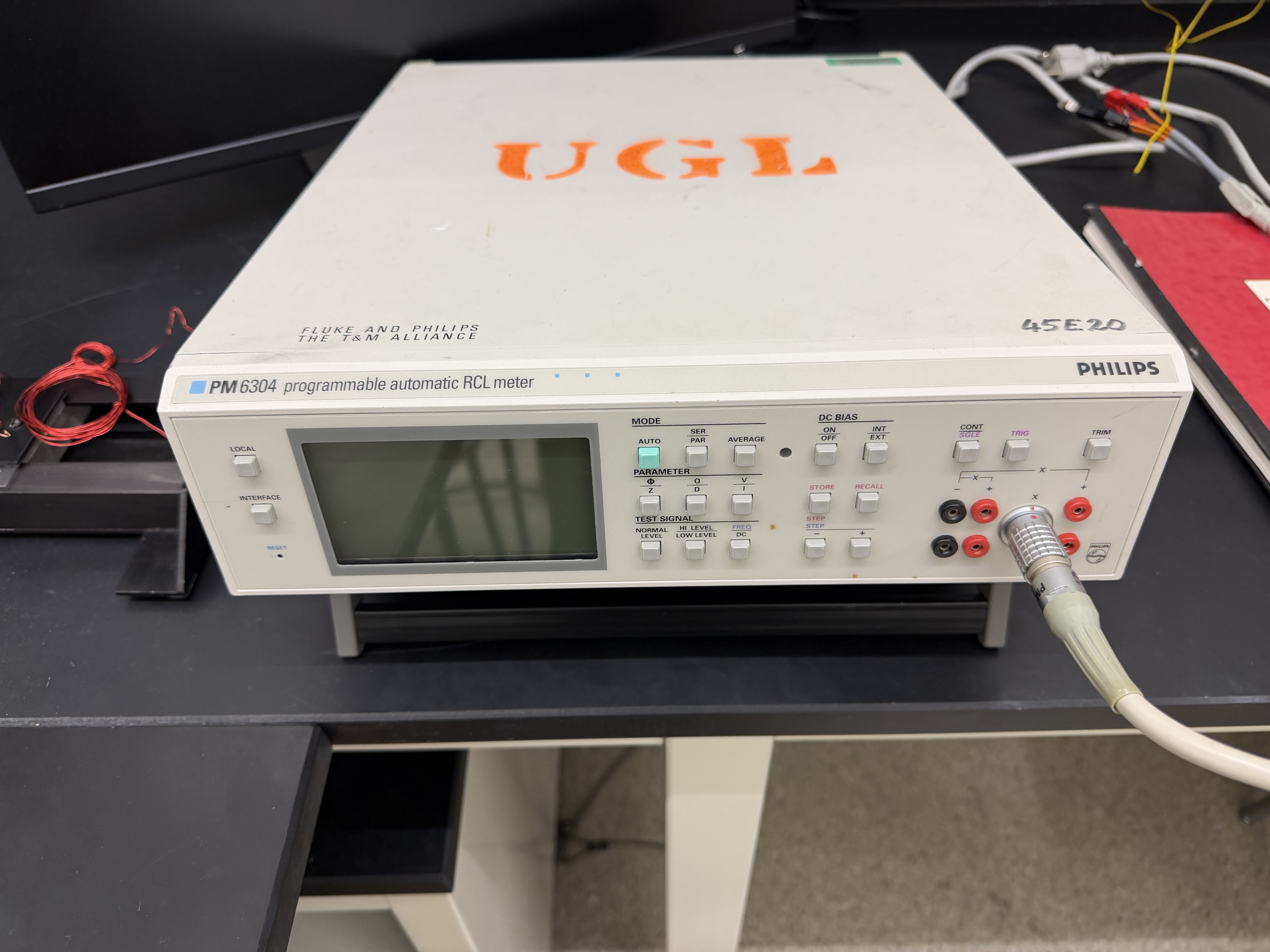
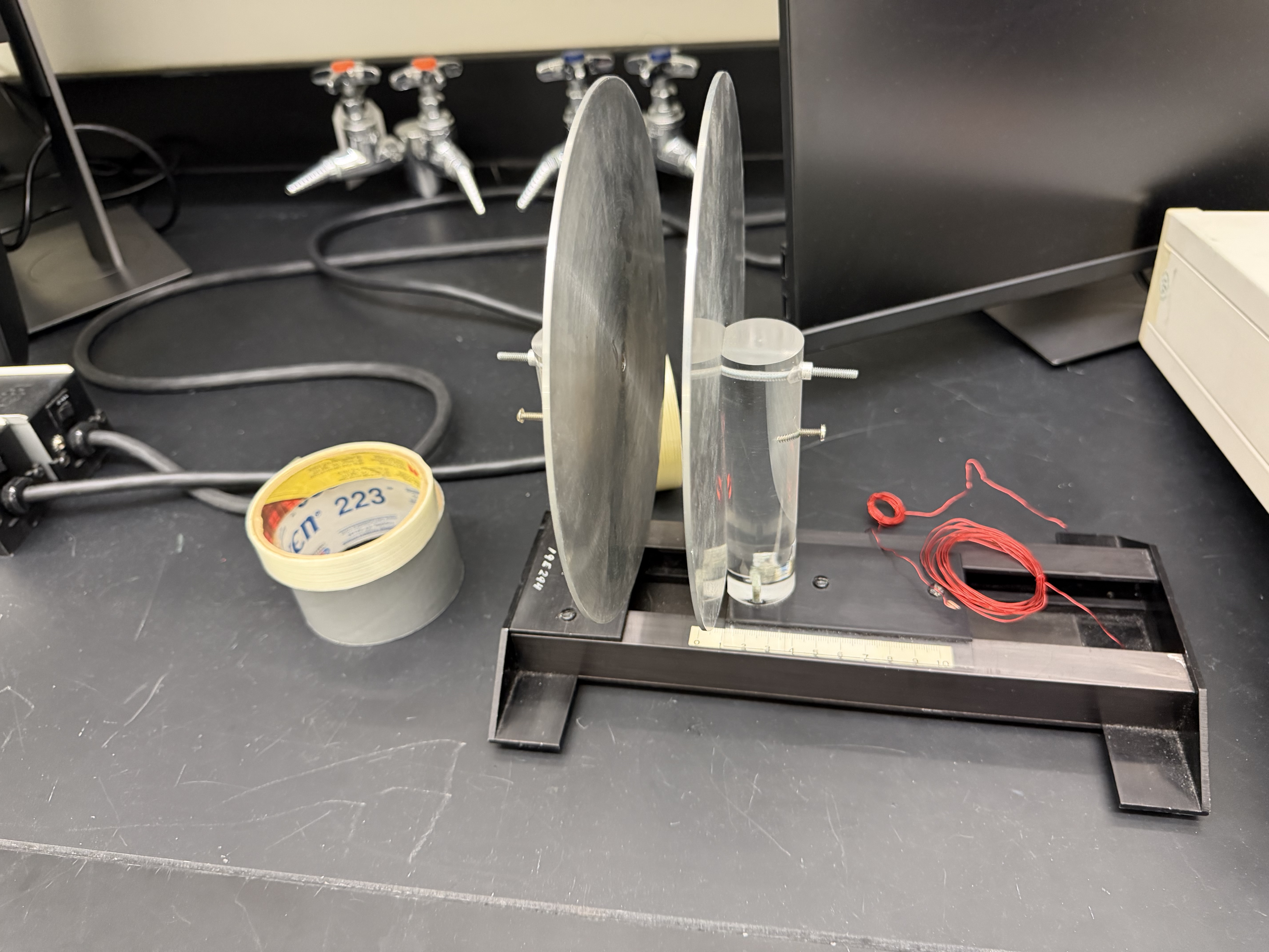
For your lab, you will use the PM 6304 RCL (see Fig. 2.1) meter to measure the conductance, capacitance and infer the critical threshold. These quantities depend on the fraction of metal to plastic beads enclosed in a volume. We’ve provided tape rolls to host your beads which you’ll place between two plates (see Fig. 2.2).
 |
 |
Week 1: Setup and Basics
For the first week, I’d like you to get familiar with your instruments and if you’re confident with your instrument, then you may start your measurements of $p_c$. The following are some questions which will come naturally as you proceed to start your experiment and therefore important to figure out at the end of this week in the lab.
Packing fraction?
Define the packing fraction $p$ as
\[p=\frac{\# \text{of metal beads}}{\# \text{of metal beads}+\# \text{of plastic beads}}.\]In theory, this is easy to compute, but the last thing you want to do is count 200 tiny metal beads before losing them accidentally, so the first logistical problem we need to figure out is a clever way to count them.
Hint: Try the weighting scale!
Conductance, Capacitance and PM 6304’s own mind
In your superconductivity lab, you’ve most likely used the fantastic PM 6304. The very versatile and convenient PM 6304 has served you well in your superconductivity lab due to its auto mode. However, in this lab, the auto mode might be something that is annoying to work as it would not be easy to know what you’re measuring.
Frequency, and Voltages and Pressure
Another thing that you will notice as you pack your beads is that the conductance changes wildly if you choose (or not) to press on the beads, i.e there is an effect of pressure on all your electrical measurements. This means that you need to apply pressure but you can’t be inconsistent otherwise it’ll mess up your data. You need to think about how to account for this.
Another important question you need to grapple with this week is the dependence of frequency and voltage. If you turn up the voltage between the plates, then sufficiently high voltages can stimulate current through the beads which affects your measurements (think about how this affects your $p_c$ for instance). Similarly high frequency also affects your measurements so you need to find a reasonable range for these quantities.
Hint: Check out this reference for ideas4
Week 2: Let’s get critical!
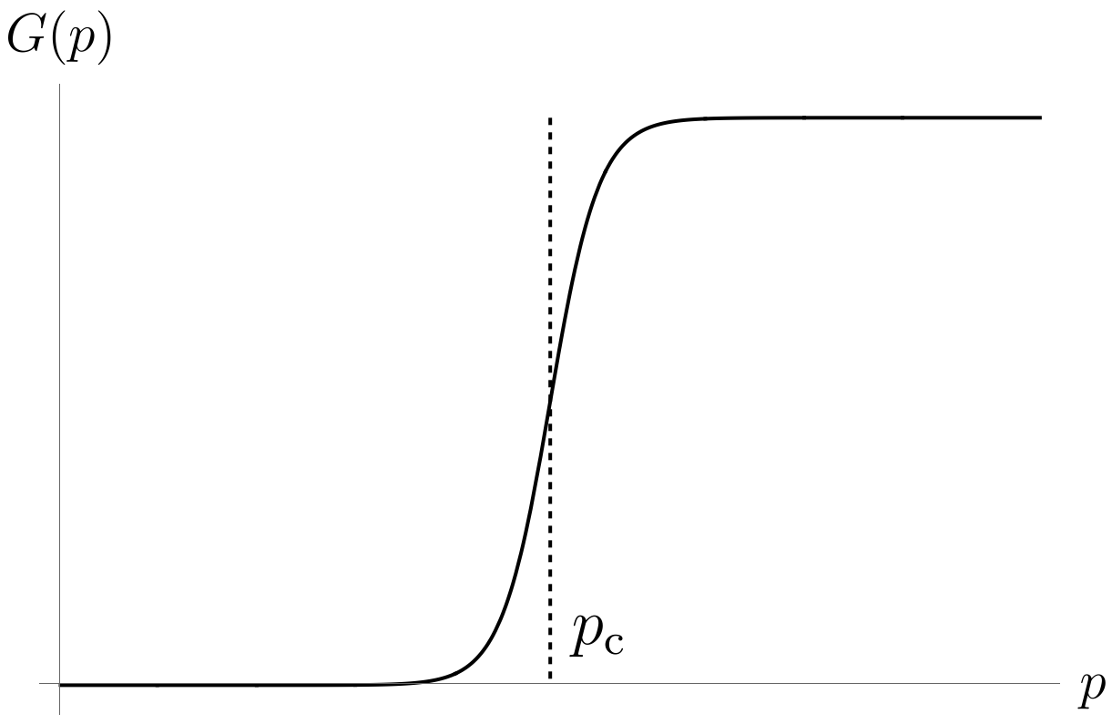
For the second week, we want to measure our observables. We’re going to measure the conductance $G(p)$ and the capacitance $C(p)$ as a function of the fraction of metal to plastic beads $p$. Your conductance measurements and capacitance measurements should look like Fig. 3.1 and Fig 3.2
 |
 |
| which you can use to deduce the critical threshold $p_{\rm c}$ which roughly corresponds to the sudden onset of conductance or divergence in the capacitance. In addition, you will also measure the admittance $ | Y(\omega) | $ at the critical threshold $p_{\rm c}$ as a function of the frequency $\omega$. After measuring $p_{\rm c}$ we will then deduce the critical exponents $t$ and $s$ by expanding about the threshold. Zooming into the critical threshold, you should find something that looks like Fig 4.1 and Fig 4.2 |
 |
 |
These exponents $s$, $t$ and $u$ can be readily extracted (using line of best fit that you’ve learnt from your previous labs) from a $\log-\log$ plot where power laws trace out a straight line with the respective slopes being these exponents.
Below are few things for you to think about:
Ensembles and statistics
“How many data points do I need?” is a question you will ask yourself during the experiment this week. Most likely, you’re thinking about varying the fraction $p$ to get a better $G$ or $C$ vs. $p$ curve. However, given a fixed $p$, is the configuration you obtain unique? Given the randomness, the probability that you get the same configuration for a fixed $p$ as your friendly colleague is highly unlikely apart from the special cases of $p={0,1}$ (which corresponds to just one configuration with all metals/plastic beads). This is why percolation belongs to statistical mechanics, the configuration you get from mixing the beads is one of many configurations you sample from an underlying distribution. It is therefore crucial that you sample more than once for fixed $p$; doing so allows you to also get error bars for your fixed $p$ measurements. You are free to decide on the number of samples you should measure, all that is required is to ensure that your measurements are statistically significant.
Why power laws?
Isn’t it remarkable that out of all the functions nature as to offer, simple power laws emerge contrasting the many-body complexity of the system? These power laws have established themselves as ubiquitous with critical phenomena and hence critical exponents. The following is an optional toy calculation to understand the origin of power laws using something called coarse-graining. It does not correspond to real 3D percolation system you’re working with as it does not produce the correct critical threshold $p_{\rm, c}$, but the ideas and the implications are the same. It is also not required for your notebook nor report, so don’t spend time on this during lab hours but If you work through it, I guarantee a highly rewarding conclusion. This exercise is divided into two parts: coarse-graining and the emergence of power laws.
Coarse-graining
Let us start with a toy model on a square lattice of size $N\times N$ with $N^2$ sites. The sites can occupy two states, which we will interpret as metal or plastic. Let $p$ be the fraction of metal beads in the system. Consider a window of size $w\times w$ that contains $w^2$ sites which divide the whole lattice into $L^2/w^2$ blocks (you may assume periodic boundary conditions if it makes the following calculation easier). For a fixed fraction $p$ and a configuration sampled from this fraction, there’s going to be some number of metal beads and plastic beads that end up in this window. You maybe tempted to conclude that the fraction of metal beads is $p$, however it turns out that is not the case. I invite you to think about why but if you don’t have a solid answer, come back to this question after you’ve finished your calculation.
We seek to understand what the effective phase of our system–is it metallic or plastic? To answer that question, we want understand how the system behaves as $w\to \infty$ for the infinite $N\to \infty$ lattice. Note that the order of limits matter here, we first take $N\to \infty$ to obtain our large system and then consider how coarse-graining affects our system. For each $w$, we coarse grain our system by assigning a simple majority rule:
Within the window $w$, if the number of metal beads forms a majority, then we replace the window with a single metal bead. Conversely, if the plastic beads form a majority, then we replace the window with a single plastic bead. Such a coarse graining procedure essentially allows us to zoom out and filter out the minutia and in essence, get a bigger picture.
Take a moment to pause and wonder what the system effectively looks like visually after coarse graining for
- $p\approx 0$
- $p \approx 1$
Now imagine slowing moving away from the extreme bounds, what do you expect to see? Make a prediction before we go ahead and attempt to compute this. For a fantastic animation of coarse-graining to help you visualize this, check out How Fractals Make the Best Coffee (11:12).
Now fixed a $p$ which implies that $p N^2$ is the total number of metal beads in the system. Let $P_{N,w}(k)$ be the probability of finding $k$ number of metal beads inside a window $w^2$ on the lattice of size $N^2$. For the majority rule, we are ultimately interested in finding \(\lim_{w\to \infty} \lim_{N\to \infty}\sum_{k>w^2/2}^{w^2}P_{N,w}(k)\) which is the probability that the window coarse grains into a metal bead if it forms a majority 5. Let’s start with $P_{N,w}(k)$ which requires us to answer the following questions
- What are the total number of ways of finding the metal beads for a fixed p on the grid?(This is your normalization factor!)
- How many ways can you populate the window of size $w^2$ with $k$ metal beads?
- How many ways can you populate the remaining sites with the remaining metal beads?
- Put 2 and 3 together, how many ways are there to find $k$ metal beads in this window?
- Finally, use 1-5 to find $P_{N,w}(k)$.
Solution
The number of ways to place $k$ metal beads inside the window that has $w^2$ sites is just \(\binom{w^2}{k}.\) However, this leaves the $N^2-w^2$ sites outside the window for grabs that we have to fill with the remaining $pN^2-k$ metal beads. The number of ways to do the latter is given by
\[\binom{N^2-w^2}{pN^2-k}.\]Doing both together allows us to faithfully uses all the $pN^2$ metal beads and account for all the $N^2$ sites. Therefore the total number of ways to find $k$ beads inside this window given that the total fraction of metal beads $p\in (0,1)$ is fixed is
\[\binom{w^2}{k}\times \binom{N^2-w^2}{pN^2-k}.\]To make this into a probability, we need to divide by the total number of configurations of the $pN^2$ metal beads on $N^2$ sites which is given by
\[\binom{N^2}{p N^2}\]Therefore, the probability of finding $k$ metal beads inside a window is given by
\(P(k)= \frac{\binom{w^2}{k}\times \binom{N^2-w^2}{pN^2-k}}{\binom{N^2}{p N^2}}\) which implies that the probability of coarse-graining into a metal bead is just
\(P(w^2\to {\rm metal\ bead})=\sum_{k>w^2/2}^{w^2} \frac{\binom{w^2}{k} \binom{N^2-w^2}{pN^2-k}}{\binom{N^2}{p N^2}}.\)
Now, we want to take the large $N$ limit and deduce \(\lim_{N\to \infty} P_{N,w}:= P_w(k).\) However, care must be exercised when taking this limit else we’ll have infinities over infinities!
- Using the definition of the binomial coefficient, write out the expression for $P_w(k)$ in terms of factorials.
- Simplify the factorials in terms of products. Use \(\frac{X!}{(X-Y)!}= (X-Y+1)(X-Y+2)\dots (X-Y+Y)=\prod_{j=1}^Y(X-Y+j)\) to make your lives easier : ).
- Factor all $N^2$ terms and perform the limit $N\to \infty$, you will find an elegant, simple sum that involves the cherished Bernoulli distribution, reminiscent of flipping coins.
This relation actual goes further: Indeed, there is an exact mapping of the $w\to \infty$ limit to the coin problem that allows us to evaluate this limit:
- What is the probability to end up with greater than $50\%$ heads as the number of flips, $n=w^2$ becomes infinite? i.,e \(P(\text{number of heads after } n \text{ flips} > n/2)\) in the limit $n\to\infty$.*
There are two different cases for you to consider
\[\lim_{w\to \infty}\sum_{k>w^2/2}^{w^2} P_w(k)=\begin{cases} ? &0<p<1/2 & \\ ? &1/2<p<1 \end{cases}.\]Solution
Now we perform $N\to \infty$ on $P(k)$ and then study how this sum grows as $w\to \infty$.
First, we make use of the fact that
\[\frac{X!}{(X-Y)!}= (X-Y+1)(X-Y+2)\dots (X-Y+Y)=\prod_{j=1}^Y(X-Y+j).\]Since $\binom{w^2}{k}$ does not depend on $N$, we keep it aside and focus on the $N$ dependent binomial terms. Using the definition
\[\binom{X}{Y}= \frac{X!}{(X-Y)! Y!},\]we have
\[\frac{\binom{N^2-w^2}{pN^2-k}}{\binom{N^2}{pN^2}}= \frac{(N^2-w^2)!}{(N^2)!} \cdot \frac{(N^2(1-p))!}{(N^2(1-p)-w^2+k)!}\cdot \frac{(pN^2)!}{(pN^2-k)!}.\]Using
\[\frac{X!}{(X-Y)!}= (X-Y+1)(X-Y+2)\dots (X-Y+Y)=\prod_{j=1}^Y(X-Y+j),\]we deduce
\[\frac{(N^2)^{w^2}}{(N^2)^{w^2}}\times (1-p +\mathcal{O}(1/N^2))^{w^2-k} (p+\mathcal{O}(1/N^2))^k.\]for some corrections $\mathcal{O}(1/N)$ that vanish as $N\to \infty$. Performing the limit gives the nice, clean result6
\[\boxed{P(w^2\to {\rm metal\ bead})=\sum_{k>w^2/2}^{w^2} \binom{w^2}{k} p^k (1-p)^{w^2-k} }\]We may evaluate this limit directly through mathematical tricks, but if we take a step back and view this as a coin-flipping problem, then the limit is easily attained! Consider for example the simple problem of flipping a biased coin with probability of heads $0<p<1$ which implies that the probability of tails is $1-p$. Suppose you flip a coin $n=5$ times (or flip $5$ coins), we may ask what is the probability that you get exactly 3 heads? There are a total of $2^5$ outcomes when you flip a coin, but all the ones that give you exactly $3$ heads are less than $2^5$. Since each flip is independent of the previous one (the coins do not talk to each other), the probability of getting a generic $3$ heads and $2$ tails outcome is $p^3 (1-p)^2$. However, the coins can be arranged in different ways that produce the same outcome–i.e there are different combinations of the $3$ heads and $2$ tails coins that still give us $3$ heads. So summing up all the probabilities gives us $\binom{5}{3} p^3(1-p)^2$ as the probability of finding $3$ heads amongst $5$ coins. Now what’s the probability of finding exactly $3$ or $4$ heads? It is just the sum of what we just calculated and the probability of finding exactly $4$ heads which is $\binom{5}{4}p^4 (1-p)^1$. See the pattern? Denote $P(X)$ the probability of observing the random variable $X$ which denotes the number of heads. The probability of finding atleast $h$ heads is given by
\(P(X\geq h)= P(X=h)+P(X=h+1)+\dots+=\sum_{k=h}^{n} \binom{n}{k} p^k (1-p)^{n-k},\) which is the exact form we had earlier! This allows us to reinterpret our math in terms of english:
\[\lim_{w\to \infty}\sum_{k> w^2/2}^{w^2} \binom{w^2}{k} p^k (1-p)^{w^2-k}= \lim_{w\to \infty} P(X> w/2).\]This translation to english allows us to readily evaluate this limit by reasoning alone: The average number of heads is given by $pn$. If $p<1/2$, then on average we will get $pn <n/2$ heads which means that getting more than half heads is very unlikely. This is particularly exemplified when you take the limit as $w\to \infty$, the probability of finding more than $n/2$ heads dwarfs in comparison and becomes infinitesimally small! Conversely, if $p>1/2$, then on average you are guaranteed to get more heads than tails which means that in the limit of tossing the coin infinitely many times you will definitely get more than $n/2$ heads so the limit evaluates to $1$7. Now let’s consider $p=1/2$. The expression becomes
\[\sum_{k>w^2/2}^{w^2} \binom{w^2}{k} \left(\frac{1}{2}\right)^{w^2}= \left(\frac{1}{2}\right)^{w^2}\sum_{k>w^2/2}^{w^2} \binom{w^2}{k}.\]The right hand side is almost exactly half (because of the symmetry of the binomial coefficients) sum of the binomial coefficients which is useful because the full sum, as you may recall is given by
\[\sum_{k=0}^{n}\binom{n}{k}=\sum_{k=0}^{n}\binom{n}{k} 1^n 1^{n-k}=(1+1)^n=2^n\]but it is missing the $k=w^2/2$ term. So lets add and subtract it! we find
\[\left(\frac{1}{2}\right)^{w^2}\sum_{k>w^2/2}^{w^2} \binom{w^2}{k}=\left(\frac{1}{2}\right)^{w^2}\left(\frac{1}{2} 2^{w^2}- \binom{w^2}{w^2/w}\right)\]which gives
\[P(X>w/2)=\frac{1}{2}- \binom{w^2}{w^2/2}2^{-w^2}.\]You can numerically verify that the last term vanishes for large $w$ and goes to zero as $w\to \infty$. But if you are curious, the term $\binom{w^2}{w^2/2}$ is called the central binomial coefficient which has the very pretty asymptotics [Eq. (3)] that involves $\pi$
\(\binom{w^2}{w^2/w}\sim \frac{4^{w^2/2}}{\sqrt{\pi w^2/2}}\) which does not grow as fast as $2^{-w^2}$ and voilà, it vanishes in the limit.
Ultimately,
\[\lim_{w\to \infty} P(X>w/2)= \frac{1}{2}\]when $p=1/2$ $\blacksquare$.
After computing these, take a moment to digest your incredible result, what does it mean? What does the system look like when you zoom out when $p<1/2$? what about when $p>1/2$? and most critically, what about when $p=1/2$? Is there anything geometric that sticks out to you about the system when $p=1/2$?
Solution
Zooming out, you find that the probability is still the same, no matter how far you zoom out. In this sense, $p_c=1/2$ is a fixed point for the system. Have a look at How Fractals Make the Best Coffee again if you’re having trouble seeing it! This is called scale invariance and it is precisely scale invariance that is the geometric magic that shows up at criticality. Now you might have noticed that the critical threshold $p_c=1/2$ is not the $p_c$ you see or expect for your system and that is because we have a toy model which works on a simple majority rule. The real percolation system does not follow a simple majority rule but rather a intertwining mess of metal beads and plastic beads which uses a more complicated method to zoom out. The process of zooming out and aggregating is called renormalization flow, the word flow here corresponds to how your parameters change under zooming out. For instance $P(X > w^2/2)$ approaches or flows to the values $1$ or $0$ for $p>1/2$ and $p<1/2$ respectively in our toy example. However, the philosophy and the mechanics of scale invariance is identical, there is a certain threshold $p_c$ for the system such that zooming out as we did before still gives us $p_c$, a fixed point.
Power laws
Having set our background on criticality, we are ready to answer why Power laws emerge. The key fact that we will use is the scale-invariance at criticality that you observed in the previous toy example. In particular, we will show that
\[\text{Power laws} \iff \text{Scale invariance}\]I will be referencing Brain Criticality - Optimizing Neural Computations (13:12), A. Kirsanov for the following argument.
So how do we quantify scale-invariance? Let us suppose that we are at criticality to begin with and define $P(x)$ as the probability of finding a cluster of size $x$. By cluster, we make the metal-bead network (or you’re familiar with the Ising model, we mean a connected group of the same spin) and by size we mean the number of beads that form a connected network. We will show that this probability follows a power law i.e
\[P(x)\sim A x^{-\gamma}\]at criticality and consequently any observables that can be computed from it using expectation values viz. the conductance or capacitance also follows a power law 8.
Imagine for a brief moment that you were able to diligently compute the probabilities of observing different clusters of sizes $P(x)$ for the entire lattice. Now suppose you zoom out so that you compute all clusters of size $2x$. A connected cluster of size $2x$ is going to be less likely than a cluster of size $x$ because there are fewer ways for a huge cluster to form than a small cluster which can be present at many locations. Therefore, $P(2x)<P(x)$ and so far this still does not give us any information about what these could be. It might be tempting to assume that scale invariance implies that $P(2x)=P(x)$, but this is not true, as the fraction of bigger clusters are necessarily going to be rarer than smaller clusters. Consider now instead the ratio or relative probability $P(2x)/P(x)$. This ratio clearly depends on the size of the cluster $x$ in normal scenarios, but at criticality, something different happens due to scale invariance. Although the individual $P(x)$ and $P(2x)$ depend on $x$, scale invariance implies that the ratio should not depend on $x$! This is because here we are free to zoom out by a factor of $2$ and since we get an identical “looking” system, our statistics is identical, but all our probabilities are shrunken by a factor (function) that depends only on your zoom factor. More precisely, we have that for any scale $k>0$ that we zoom out,
\[\frac{P(kx)}{P(x)}= g(k)\]for a “nice” (smooth) function $g(k)$ which, importantly only depends on $k$!
Another way to see this is through the observation that our statistics when zooming out by a factor of $k$, is identical to what we had (because we see similar looking clusters) except that all our probabilities are scaled by some function that depends on how much we’ve zoomed out, i.e
Infact, the above two equations are the definition of scale invariance and can be used if one has scale invariance. You can easily see power laws $\implies$ scale invariance by plugging in a generic power law to obtain the above equation. The converse however is non-trivial, but the fantastic result above and some calculus is all we need to show power laws–which I will walk you through with the following exercise.
- Assume that $P$ is a smooth function, differentiate Eq. 1 with respect to $k$ and set $k=1$.
- Solve the resultant ODE for $P(x)$ 9.
- Call $g^\prime(1)=-\gamma$, what functional form do you find for $P(x)$?
After an interesting cocktail of combinatorics and calculus, and the simple idea of scale invariance at criticality, we have derived the emergence of power laws. This is why power laws are ubiquitous with critical phenomena.
Solution
Observe that
\[\frac{P^\prime(x)}{P(x)}= \frac{1}{x}g^{\prime}(1)\]which can be solved to obtain
\[\ln(p(x))=-\gamma \ln(x)+C\]for some integration constant $C$ which upon exponentiating gives
\[P(x)= \underbrace{e^C}_{=A} e^{-\ln(x)\gamma}= A x^{-\gamma},\]that is a power law $\blacksquare$.
Week 3: Universality and Scaling Theory
For the final week, we want to study the consequences of scaling theory and universality. In addition to the conductance and capacitance measurements, we will measure the admittance exponent $u$ and test the prediction from scaling theory \(u=\frac{t}{t+s}\) and \(\delta_{\rm c}=\frac{\pi}{2}(1-u)=\frac{\pi}{2}\frac{s}{s+t}\) where critical loss angle $\delta_{\rm c}$ is defined to be the angle $\delta=\delta_{\rm c}$ in the dissipation factor $D=\tan(\delta)$10
In the abstract we motivated our experiment with the notion of universality, but what exactly is this universality in the context our phase transitions? To begin to answer this question, let us start with identifying what is not universal in our system. There are two critical things in our experiment, the critical exponents and the critical threshold, it turns out that the exponents are universal but the threshold $p_{\rm c}$ is not. Here are some experimental & theoretical (computational) results for the percolation threshold $p_{\rm c}$ for a few lattices across dimensions $d=2,3$.
| Dimension | Lattice | Percolation threshold |
|---|---|---|
| $2$ | Square 11 12 | $0.5923(7)$13 |
| $2$ | Honeycomb 12 | $0.6962(6)$ |
| $3$ | Cubic 14 | $0.3116077(2)$ |
| $3$ | Randomly Packed Hard Spheres (RPHS)15 16 | $ 0.310(5) $ |
Notice that the threshold for the Square and Honeycomb lattice are very different however, notice that the threshold for the RPHS (which is what we have) is very close to the cubic lattice. This is actually quite unexpected, the former is a random mess whereas the latter is a uniform regular lattice. In the context of percolation, since the threshold is not universal, a natural question one might immediately ask upon a threshold result is “what is the underlying lattice?”.
Now let’s think about what is universal about our system. The theory of phase transitions is dedicated to understanding the different phases that arise when certain parameters change. A canonical example of a phase transition is that of water to ice over a temperature range or that of the para-ferro magnetic transition after a critical temperature 17. A mathematical object is needed to characterize the different phases, something that is $0$ when it is in one phase and $\neq 0$ when it is in the phase you care about18. Such a quantity is called an order parameter
Order parameter $(\Psi)$: A number used to quantify two different phases that arise when changing a parameter $\zeta$, $\Psi(\zeta)=0$ below a critical threshold $\zeta<\zeta_{\rm c}$ and $\Psi(\zeta)>0$ for above $\zeta>\zeta_{\rm c}$.
In the standard Bernoulli percolation problem with fraction of connected links $p$, the order parameter is given by $\Psi(p)=\mathbb{P}_p[O\leftrightarrow \infty]$ where
\[\mathbb{P}_p[O\leftrightarrow \infty ]: \text{Probability } \exists \text{ connected cluster from the origin to far off infinity at } p\]The origin $O$ is an arbitrary site and far off infinity means the boundary of your large system. For low $p\approx 0$, none of them make it to the end, but for $p\approx 1$, most if not all of them form clusters that reach the boundary, after the critical value $p_{\rm c}$ it shows a sudden change 1 3. Expanding about $p=p_{\rm c}$ we find that the order parameter scales with an exponent \(\mathbb{P}_p[0\leftrightarrow \infty]\sim (p-p_{\rm c})^\beta,\) where $\beta$ (called the beta exponent) is the critical exponent for the (canonical) order parameter which is universal! In two-dimensions, no matter what lattice you use, there is an exact and spectacular and universal number for this exponent
\[\beta=\frac{5}{36}.\]In our experiment, we look at the critical exponents $t$ and $s$ which is not $\beta$. Accordingly, one may find other exponents viz. $\nu$, the correlation length exponent or $\gamma$, the mean cluster exponent or $d_{\rm f}$, the fractal dimension. For details check out the wiki. For two-dimensional Bernoulli percolation, the exponents are given by rational numbers
| $d$ | $\beta$ | $\nu$ | $d_{\rm f}$ | $\gamma$ |
|---|---|---|---|---|
| $2$ | $\frac{5}{36}$ | $\frac{4}{3}$ | $\frac{91}{48}$ | $\frac{43}{18}$ |
Aside from the universality of these exponents, what is even more interesting is that these exponents are not independent of each other. Indeed, they satisfy the so-called scaling relationships (if dimension $d$ enters the equation, it is called a hyper-scaling relationship). One of these scaling relations includes the fractal dimension $d_f$, the dimension $d$ alongside $\beta$ and $\nu$ which satisfy \(d_{\rm f}= d- \frac{\beta}{\nu},\) that you may readily verify from the table above! These scaling relationships are in a sense more universal than the already universal exponents themselves and hints are a deeper connection between dimensions and topology in phase transitions.
Few things to think about:
Why is $p_{\rm c}(\text{RPHS})\approx p_{\rm c}(\text{Cubic})$?
The observation that these non-universal thresholds are so close requires some investigation.
Hint: Check out the references!
How does one measure $\beta$?
The canonical order parameter is the probability $\mathbb{P}[0\leftrightarrow \infty]$ that we mentioned earlier with the exponent $\beta$. Unfortunately, we do not measure $\beta$ in our experiments but that leaves the natural question: How does one measure $\beta$ for a three-dimensional system in the first place? Although $\beta$ is a nice rational number in $2$-d, what is its (numerical) value in $3$-d?19
Admittance and frequency range
How can one easily deduce the admittance from the 6304? What frequency range should you work with at $p_{\rm c}$?
Error propagation and comparisons
Ensure to propagate all quantities that are composed of quantities that have error. For instance, the theoretical prediction of $u=\frac{t}{t+s}$ should have an error that comes from your observed value with their errors $t\pm\delta t$ and $s\pm \delta s$. Measuring $u$ directly from the experiment through a $\log-\log$ plot is accompanied by an error from the fit that should be included.
Scaling theory and predicting $u$
Below is an optional exercise to get a taste of scaling theory which predicts what the exponent $u$. We use observation that the admittance is non-zero and finite at $p=p_{\rm c}$ and depends on $\omega$. I will be referencing 6. The Scaling Hypothesis Part 1, M. Kardar.
We begin by considering the frequency dependent complex admittance $Y(\omega,p)$ which contains both the conductance and capacitance defined by
\[Y(\omega,p):= G(\omega,p)+i \omega C(\omega,p)\]Electronically, the metal-plastic bead system is equivalent to an RC circuit with effective resistance $R$ and capacitance $C$ (both of which you measure) that sets a characteristic frequency scale $\omega_{0}$.
- Recall and state the characteristic frequency scale $\omega_0$ for an RC circuit. Using $G=1/R$, express $\omega_0$ in terms of the conductance $G$.
Now, the admittance also depends strongly on the fraction $p$. If you look the graphs for $G(p)$ and $C(p)$, we notice that just above the percolation threshold, the capacitance decays while the conductance grows rapidly (limited only by the fact that the beads have some contact resistance). Conversely, just below the threshold, the capacitance grows rapidly whereas the conductance is tiny. We can reframe our observation as
\[Y(\omega,p)\sim \begin{cases} A (p-p_{\rm c})^t & p> p_{\rm c}, \\ i B \omega |p-p_{\rm c}|^{-s} & p <p_{\rm c} \end{cases}\]where the factors $A$ and $B$ are used to ensure that the dimensions work out ($A$ has units of conductance, siemens). Now we may imagine trying to write this as a single expression and imagine we factor the sign independent $(p-p_{\rm c})^t$ from it to get
\[Y(\omega,p) \sim A |p-p_{\rm c}|^t \times (\text{some dimensionless function for } p> \text{and }p< p_{\rm c}).\]which has the same scaling when $p>p_{\rm c}$. Note the dimensionless nature of this new function. This new function should have as an input
- something that depends on the frequency $\omega$ but dimensionless
- something that depends on $p-p_{\rm c}$ with some arbitrary exponent
Denote $\omega_0$ the natural frequency scale set by our system and let $\phi$ be this arbitrary exponent. This gives us that the scaling function $g_{\pm}$ should assume the form
\[Y(\omega,p)\sim A |p-p_{\rm c}|^t \times g_{\pm} \left(\frac{\omega}{\omega_0} |p-p_{\rm c}|^\phi \right)\]where $g_{+}$ is the scaling function for $p-p_{\rm c}>0$ and $g_{-}$ for $p-p_{\rm c}<0$ both depending on the dimensionless variable $x=\frac{\omega}{\omega_0} |p-p_{\rm c}|^{\phi}$.
-
Assume that $p>p_{\rm c}$, in the small frequency limit $\omega\to 0$ (remember that by “small” $\omega$ we mean $\omega \ll \omega_0 $), we should have $Y(\omega,p)\sim A |p-p_{\rm c}|^t$. Given this, what should the $\lim_{x\to 0} g_{+}(x)$ become in order to match what we should have? (you don’t need to find the exact value of $g(0)$, but rather only identify and choose if it should be a power law, a constant, a divergence or an exponential.)
-
Conversely, given that $p<p_{\rm c}$, what should $\lim_{x\to 0}g_{-}$ grow like to match $\omega |p-p_{\rm c}|^{-s}?$ Use this matching condition to derive $\phi=-(s+t)$.
Now that we have $\phi$, the general form reads
\[Y(\omega,p)\sim A |p-p_{\rm c}|^t g_{\pm}\left(\frac{\omega/\omega_0}{|p-p_{\rm c}|^{(s+t)} }\right)\]Since $s,t>0$, at criticality, $|p-p_{\rm c}|^{-(s+t)}\to \infty$ when $|p-p_{\rm c}|\to 0$. But experimentally we know (or you will find) that $Y(\omega,p)\sim (i \omega)^u$ for some exponent $u$. The key fact to keep in mind is that $Y(\omega,p_{\rm c})$ is neither zero nor infinite. Since $|p-p_{\rm c}|^t \to 0$ but $\frac{1}{|p-p_{\rm c}|^{s+t}}\to \infty$ as $|p-p_{\rm c}|\to 0$, we have two competing limits that requires some care.
4. To obtain a finite limit for $Y$, we need $g_{\pm} (x)$ to grow. Suppose that it grows in the following manner $\lim_{x\to \infty} g(x)\sim x^q$ for some exponent $q$. Match the limit with $Y(\omega,p_{\rm c})\sim i \omega^u$. What do you get for $q$? Using the fact that $Y$ is neither infinite nor zero, obtain the scaling relation \(u= \frac{t}{s+t}\)
Finally, now we deduce the critical angle $\delta_{\rm c}$. The loss tangent is defined as
\[\tan(\delta)= \frac{G}{\omega C}\]5. Using $Y= G + i \omega C= (i\omega)^u$ and Euler’s identity, find $G$ and $C$ in terms of $u$ and express $\tan(\delta)$ in terms of $u$. The resultant angle is our critical angle!
With essentially what’s Dimensional Analysis part II, you have derived your first scaling relation! Congratulations! Now go forth and test your prediction. If you liked this calculation, you invite you to check out M. Kardar’s lecture video that I cited.
-
Fantastic expository talk by Fields medalist H. Duminil-Copin ↩ ↩2
-
Veritasium video on avalanches, forest fires, universality and criticality ↩
-
Bernoulli percolation: A more mathematical dive into percolation ↩ ↩2
-
D. Dziob; D. Sokołowska, Experiment on percolation for Introductory Physics Laboratories —A case study Am. J. Phys. 88, 456–464 (2020) ↩
-
The term $w^2/2$ evaluates to a non-integer solution if $w$ is odd. However since we are ultimately interested in the limit of large $w$, you may freely choose $w$ such that $w^2/2$ is an integer. ↩
-
I’d like to thank my friend and colleague Connor Walsh for working on this calculation together! ↩
-
The astute amongst you might recognize that the average does not wholly characterize the distribution because the width $\sigma=\sqrt{n p (1-p)}$ (i.e the standard deviation) can characterize the non-zero probability of finding $n/2$ heads after $n$ flips. So on average you will find $np \pm \sqrt{np (1-p)}$. However, what matters is the signal-to-noise ratio or size of the mean with respect to $\sigma$ which gives $np/\sigma\to 0$ as $n\to \infty$ meaning that the width is so negligible that it is not sufficient to get you above $n/2$. ↩
-
This is because the expectation values are essentially integrals and integrals of power laws are still power laws if the exponent is not $-1$. ↩
-
To avoid notational ambiguity, recall for instance if $f(\zeta)=\sin(\zeta)$, then $f^\prime(\zeta)= (f^\prime)\circ \zeta= \cos(\zeta)$, i.e $P^\prime(x)$ is just another function that is evaluated at the input $x$ ↩
-
Yes, the same D in PM 6304 ↩
-
T Gebele 1984, Site percolation threshold for square lattice J. Phys. A: Math. Gen. 17 L51 ↩
-
Z V Djordjevic et al, Site percolation threshold for honeycomb and square lattices J. Phys. A: Math. Gen. 15 L405 (1982) ↩ ↩2
-
$0.5923(7)$ is equivalent to $0.5923\pm 0.0007$ ↩
-
J.Wang, Z. Zhou, W. Zhang, T. M. Garoni2, and Y. Deng, Bond and site percolation in three dimensions Phys. Rev. E 87, 052107 (2013) ↩
-
M.J. Powell, Site percolation in randomly packed spheres, Phys. Rev. B 20, 4194 (1979) ↩
-
H Ottavi et al, Electrical conductivity of a mixture of conducting and insulating spheres: an application of some percolation concepts, J. Phys. C: Solid State Phys. 11 1311 ↩
-
Although these phenomena are examples of a phase transition, the water-ice transition is an example of a first order phase transition whereas the para-ferro magnetic transition is an example of a second order transition. The terms “first” and “second” are now archaic, often interchanged by the terms “discontinuous” or “continuous” respectively in the modern lingo. ↩
-
For more sophisticated systems, the order parameter can be a complex number, a vector or even a matrix (perhaps with complex numbers!) ↩
-
It is an open question whether $\beta$ admits a rational form, people have looked for decades but have not found it (yet!) ↩