Thermal Energy

The fundamental insight from the Franck-Hertz experiment is that of discrete energy levels. When electrons that are accelerated across a potential difference attains a “critical” energy and “collide” with Hg atoms, something magical happens– a sudden transfer of energy! This is precisely what you’re observing when you increase your accelerating voltage $V_a$ and obtain these peaks in the collector current (although with many many electrons). Recall that an electron moving across a potential difference of $V_a$ attains an energy of $e V_a$. For example: if $V_a=5V$, then the electron gains an energy of $5eV$ after crossing over the potential difference.

Simultaneously, we know that turning up the temperature makes atoms jiggle, i.e, they gain energy. Imagine setting $V_a=5V$, you would then naturally conclude that the energy gained by an electron is $5 eV$. But wait! if these electrons also move due to temperature, surely they must gain some thermal energy right? Even though your power supply reads $5.0 V$, how sure are you that the thermal energy doesn’t change the expected energy to, say $(5\pm 2)eV$ instead of $5 eV$?

In other words, how relevant are these temperature effects to the energy?

What's happening?

As a physicist, a way to think about the question of “relevance” is that of scales. In nature, there are time scales, length scales and energy scales. What therefore matters is not the minute details, but the order of magnitude. The difference in these scales generally requires different models and, in a nutshell, is also what makes physics hard!

In our problem, let’s compare the energy scales of thermal noise with the energy supplied (i.e electron volts). Whatever sources you look up for the energy due to thermal noise, you will find that the thermal energy $E_T$ at temperature $T$ is roughly \(E_T \sim k_B T.\)

Given that your operating temperature is $T=180^\circ C$, an order of magnitude estimation gives \(T\sim 10^2 K.\)

The Boltzmann constant $k_B$ has units of $\frac{\rm Energy}{\rm Temperature}$, and can be written in terms of $eV/K$ as

\[k_B= 8.6 \times 10^{-5}eV/K\sim 10^{-4} eV/JK\]

i.e the thermal noise is roughly \(E_T\sim 10^{-2} eV.\)

What this means is that any fluctuations you see will be on the 2nd decimal place to your right which is beyond the range that the FH power supply can work up to!

However, this is not the end to our story, thermal effects do play a role in our measurements but are negligible for the peaks at high $V_a$. Specifically, the filament temperature is around $T_f\sim 10^3 {\rm K}$ which affects the first peak as the thermal fluctuations contribute $E_{T}\sim 0.1 eV$ that competes against the smallest increment in your power supply.

Energy Levels?

You’re diligently doing your Franck-Hertz experiment, imagining the electrons colliding with the mercury atoms and transferring their energy to the atoms by exciting them to the “next energy level” until you ask yourself “what are these energy levels and what do they correspond to?”

You’ve learnt about the Bohr model and decide to estimate this difference in the energy between these energy levels–surely the difference should be the same energy that the electrons transfer right? So you pull up the atomic configuration of mercury and find that last electron is at the $n=6$ energy level. The next state is at $n=7$, so the difference in the energy should be

\[E_{7}-E_{6}= -13.6 eV Z^2 \cdot \left(\frac{1}{7^2}-\frac{1}{6^2}\right)\approx 641 eV,\]

where you have used the atomic number of mercury $Z=80$ and therefore the nucleus has a positive charge of approximately $80 e$.

Then you realize that something is wrong with your calculation: It is two orders of magnitude bigger than what you expect! What’s wrong? Could it be that there are missing energy levels? if so, where or what are they?

What's happening?

The Bohr model, that’s the problem! Specifically, the Bohr model is only valid for hydrogen-like atoms and our Hg atom is the last thing that is close to being hydrogen-like. However, most chemists uses hydrogen-like orbitals to do chemistry; the “s,p,d,f” orbitals we talk about are all solutions to the hydrogen atom shoe horned onto heavier atoms, so what gives? Start with the hydrogen atom which has one electron and a proton, the Bohr model tells us that the ground state corresponds to \(n=1\). The index “n” is what we call a quantum number and describes a quantum state. What’s interesting is that the solutions of the Schrödinger equation (for the hydrogen atom) produces new quantum numbers \(\ell\) and \(m\) from conservation of angular momentum. The states with \(\ell=0\) are what we call the “s” orbitals and the other funny letters are for \(\ell \geq 1\). So in the atomic configuration of H, we find

\[[{\rm H}]= 1 s^1,\]

which is meant to be read as a state which has one electron in the so-called “s” shell in the \(n=1\) state. So if there are states labelled by different quantum numbers, then shouldn’t they have different energies contradicting the formula \(E_{n}= -13.6 {\rm eV}/n^2\)? It turns out that for the hydrogen atom, we’ve got a degeneracy! the energy levels only depend on the quantum number \(n\).

The story is different in the case of the atomic configuration of Hg in which you’ll find

\[[{\rm Hg}]= [{\rm Xe}]\ 4f^{14}\ 5d^{10}\ 6s^2.\]

The configuration tell us that that the outermost shell \(n=6\) contains two electrons in the “s” shell and is described succinctly as \(6s^2\). For non hydrogen-like atoms, the energy degeneracy is lifted due to the simple fact that the energetics depend on the electron-electron interaction! Coulomb repulsion forces electrons to optimize between the attractive force of the nucleus and the repulsive force from their neighbors making them occupy these other orbitals between \(n=6\) and \(n=7\) shells. These orbitals in between, too, are an approximation. Atomic physicists use something called term symbols to describe the states which you can find if you search energy level diagrams for your atom, but the main takeaway here is that “missing” different energy levels that were always present in the background for the hydrogen atom but washed away due to degeneracy arise from the coulomb repulsion between many electrons. This many-body interaction is precisely what makes Quantum mechanics so hard!

Before we conclude, I’d like to point out the fact that although Quantum mechanics is hard, that does not halt nature in displaying these discrete energy levels. Without the calculations, one can still observe these energy levels through the spectral lines. As you know, Franck and Hertz noticed that the spacing between the peaks was roughly $5{\rm eV}$. What was extraordinary was not this realization, but the fact that they computed the corresponding emission wavelength and found that it is $253.7 {\rm nm}$ or $2536 {\rm Angstrom}$. They then compared it to the spectral lines of mercury gas and found that this same line was present. They hypothesized that this was the only transition in the FH apparatus, so they tested it within the apparatus and found something incredible. I will just show you what they found and have you take in what it means.

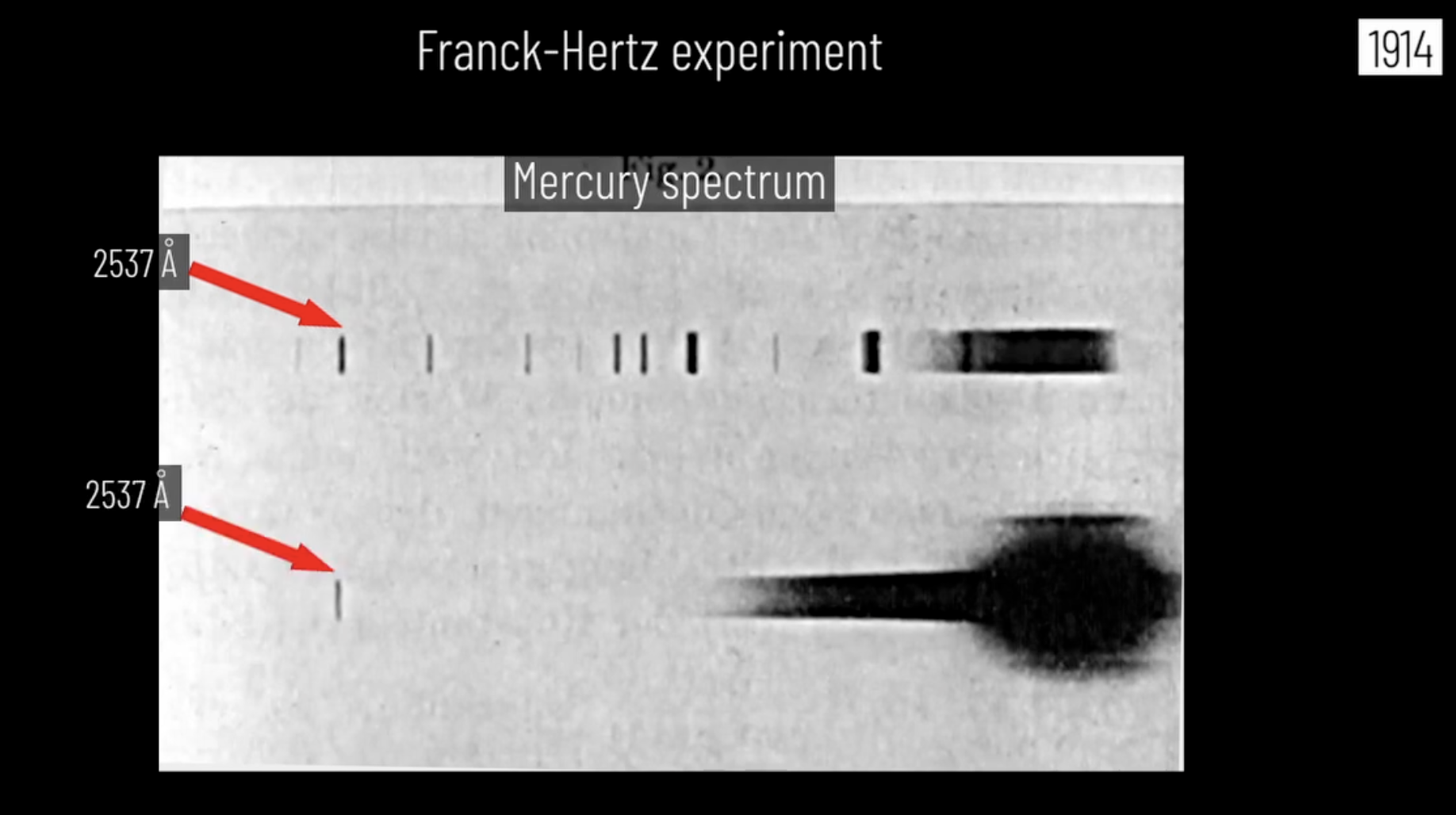
Image credits: Dr. Jorge S. Diaz from J. Franck’s Nobel Lecture

Fitting data

You’re finishing up the Franck-Hertz experiment, almost done with this hectic lab. By now you’ve got a comfortable grip on your apparatus and you’ve seen the troughs and peaks at roughly \(5 {\rm eV}\) intervals–congrats on doing some cool science! Now that the experimental aspects are over, you move to your analysis. Earlier you observed “roughly” \(5 {\rm eV}\), but can you do better? You want to find the exact location (value of \(V_a\)) of the troughs (or peaks) to see the difference clearly. As a first order approximation, you might look for the smallest (biggest) current or amplitude from Logger Pro within a certain range and identify that as the trough (peak).

But, as you zoom into the trough (peak), the illusion of a smooth continuous curve vanishes, you’re left with discrete points. In the very unlikely case that your smallest (biggest) current corresponds to the real trough (peak) location, you’re golden. However, the most likely scenario is that the resolution you have wasn’t fine enough to obtain the exact trough (peak). For example, two points were recorded with some width \(\Delta V\) such that the real trough (peak) is in between them. Additionally, all this hinges on the fact that the \(I\) vs \(V\) curve you measured is constant over trials, but, as you’ve noticed during your sweep up (\(V_a:0\to 65 V\)) and down, the curves do not lie on top of each other–Why conform to a fixed curve when another measurement produces a slightly different curve? So you need to package the different current values you get with multiple trials as an uncertainty in your current measurement.

In these cases when you’ve got missing data points, you need to perform a fit. A fit extrapolates the data you measured using a particular model (linear, exponential etc) and outputs the parameters used in the model. In your case, the parameters you’re looking for are the location (\(V_a\)) of the trough (peak) and a characteristic width. Although the fit takes care of one data set, you need to simultaneously account for error in your current measurement to address the different possible data sets you might get over different trials.

Therefore the natural questions you need to ask now are

1. What fit do I use?
2. Given this fit, how do I estimate the (current) errors?

Note: As part of the analysis, you need to perform a fit and a \(\chi^2\) test for your fits. Refer lecture notes for the details on how to do both. If you seek intuition on this whole fitting business, feel free to check out some stuff I wrote on Least-squares and fitting curves through points and What the heck is \(\chi^2\) anyway?.

What's happening?

Think about it!