Science
Lesson 5: Whispering gallery modes
lesson1 lesson 2 lesson 3 lesson 4
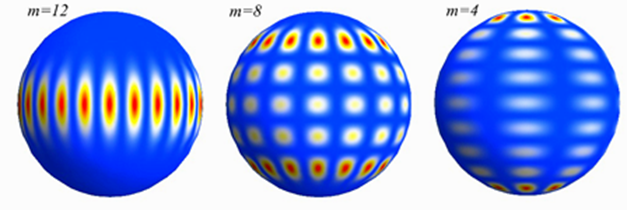
The images above are 3D plots of the electric field corresponding to three different whispering gallery mode resonances of one of our glass microspheres. Beautiful, no?
One can do other cool things, like calculate the oscillations of the optical field. We can't actually see these, because they happen trillions of times a second. But if you go back the standing waves on a string in the first page, this movie is the same thing, but for an optical resonance.
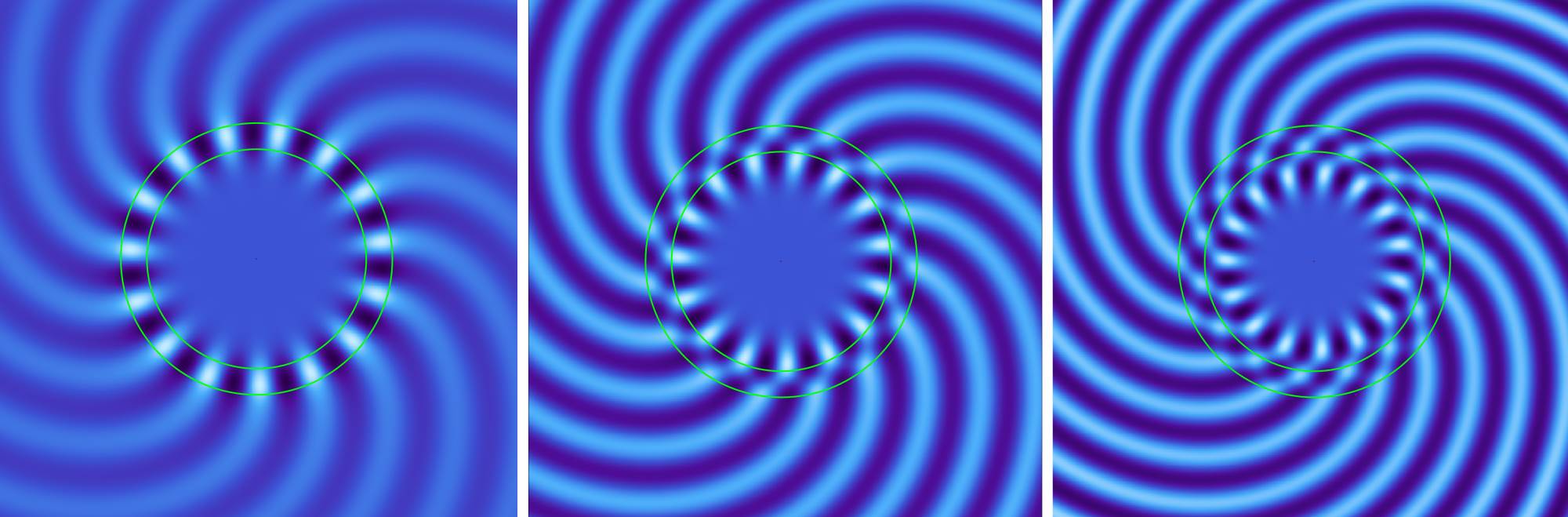
The two red circles in the image define three regions. The inner region is a glass sphere. The middle region (between the lines) represents a fluorescent coating of the kind we make in our research. And the outer region is air.
This time, you might notice that the resonant energy isn't confined inside the gallery. It actually radiates outward and interacts with the surrounding medium. This gives us a chance to use these resonances for microscale sensing applications. Some of these are discussed on the research page.
Finally, let's get a little more technical and talk about some of the important properties associated with all resonances, but especially the whispering gallery mode optical resonances described above.
Q-factors
The quality (Q) factor is one of the two most important properties of optical resonances in any kind of cavity (the other is the optical mode volume, which we will also discuss). Q-factors are a direct measure of the ability of the cavity to confine and store light. Higher Q-factors mean the cavity confines the energy inside more effectively, and will produce stronger effects on light trapped inside.
Mathematically, the Q-factor has a number of simple definitions. It is technically proportional to the ratio of the optical energy stored in the cavity to the energy lost per oscillation cycle. So, a high Q-factor means a lot of optical energy stored in the cavity with very little loss. The same thing is, of course, true for any type of resonating cavity - even a standing wave on a fixed string.
Unless you do certain specialized techniques called "ringdown spectroscopy", it can be very hard to figure out how much energy is lost in your cavity per cycle. For example, in our work all we normally see is a fluorescence spectrum with a bunch of peaks in it where the resonant modes are. Luckily, there is a simpler, equivalent definition that lets us work out the Q-factors. In this definition, the Q-factor is simply the ratio of resonance frequency divided by the resonance linewidth. Although it may not seem like it, this is a direct consequence of the first definition and can be proven mathematically.
We've measured Q-factors approaching one billion in spheres without a fluorescent coating, and about one million in quantum-dot-coated spheres.
Mode volume
The mode volume is a slightly more difficult concept than the Q-factor. Essentially, the mode volume is a measure of the spatial confinement of electromagnetic radiation inside the cavity. Just like a higher Q factor will lead to stronger cavity effects, so does a smaller mode volume.
Mathematically, the mode volume is defined as the volume integral of the electric field intensity in and around the cavity, normalized to the maximum field intensity (the latter means that the mode volume does not depend on the magnitude of the field itself). This implies that we are integrating the electric field intensity over all space. The problem is, these are "open resonators" - that is, energy leaks out into space. This is different from the conventional solutions for closed resonator cases such as a vibrating drumhead, and it makes the physics a bit more complicated. For an open resonator we can set an integration limit at some reasonable value, such as 100 times the cavity radius. Obviously, this is an approximation that improves as the integral extends further out, but unfortunately it diverges at infinity. This is the "traditional" problem of an open resonator, and it means the mode volume should be though of as approximate.
So the ways that the fluorescent quantum dots interact with the microcavity are controlled largely by the mode volume and Q-factor of the cavity, and by the emission properties and geometry of the dot inside the cavity. In our case, we typically deal with cavities having a circular symmetry, such as rings, disks, or spheres. The QDs are generally at or very close to the WGM electric field maximum, which is the optimal location. Thus, we can observe very strong, intense resonances in the emission spectra.
In the image below, you can see how the field intensity looks for a WGM of a sphere (in cross section). The color represents field amplitude. If you know something about modes already, these are three different counterclockwise-propagating TE-polarized radial modes. The mode volume in this case is very large and extends well outside the cavity, which is important for sensing applications.
Sensors
First, let's talk microcavities again. The exact wavelength at which these resonances occur can be sensitive to the nature of the medium surrounding the microcavity (both its refractive index and absorption). In the simplest cases, the sensing action is simply a refractometric effect: as you change the refractive index outside the cavity, the mode resonant positions shift. We can measure these shifts to determine the change in refractive index of a fluid medium.
In our work, we have a thin layer of fluorescent quantum dots coating the surface of a sphere or capillary channel. The way we get the quantum dots into the capillary is the subject of a patent.
For a sphere, the analyte fluid medium needs to be on the outside. But for a capillary, it is on the inside. In either case, a fraction of the resonant field energy must extend into the analyte region for sensing applications.
For a capillary structure, the WGMs are confined by the QD layer but they extend slightly into the interior channel, thus enabling fluid sensing. Analytes are pumped through the capillary core using a micro-syringe pump and the fluorescence WGM positions measured with a spectrometer. This combines microfluidics with quantum-dot detection methods.
We've used this method for detecting refractive changes due to the addition of a variety of solutes in water; for example, sucrose, glucose, alcohols, heavy oils, and other chemicals. We are now turning to mixtures of oil and water, and also true biosensing using surface functionalization chemistry. All this really means is that by treating the channel surface (the QD film) with certain chemistry, we can make target biomolecules preferentially stick to the sensing surface. Microfluidic biosensing of this type is likely to be important in a wide variety of technologies, from medical diagnostics to environmental monitoring and control.
So, that's a short summary of the science. Obviously, one could write a book to describe everything. Some microcavity books have been written but they unfortunately tend to be very technical and quite hard to follow unless you've already got a fair bit of expertise in the field. Someday, someone will have to write a good book on microcavities, as they are becoming more and more important in optics, photonics, sensing, microlasers, and other applications. Meanwhile, feel free to send me any comments you may have!