Secondary Analysis

Choice of Analytical Techniques

The initial intent of this project was to examine the influence of a range of anthropogenic disturbances on riparian and wetland associated bird communities at multiple scales. Given the dataset is not yet complete for all environmental variables at all scales (see Data Preparation below)I could not use the multiscale approach. Some preliminary analysis using distance-based Multivariate Regression Trees (db-MRT) (1) in Program R suggested that anthropogenic disturbance variables may account for up to 40% of the variance in the dissimilarity matrix (Bray Curtis) used to summarize the community composition data. A potentially powerful exploratory analysis and predictive technique, db- MRT uses hierarchical partitioning to select the most important variable that best explains the construction of the dissimilarity matrix (1;2). Once a split is made another variable is selected that best explains some cutoff in the reaminaing data. These splits are then displayed in a tree that resembles those produced in cluster analysis but with each node representing a cutoff value of an explanatory variable(2). Because the analysis considers only one variable at a time issues of collinearity are avoided. Unfortunately, this technique does not allow for use of covariables. Thus, controlling for variance explained by habitat variables is not possible. As a result, I had hoped that partial RDA or CCA would be robust enough to partition the variance in community composition explained by each of the disturbance variables (Table 2).

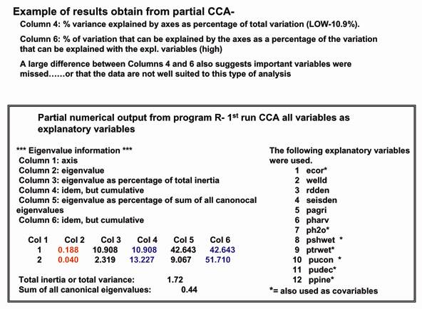
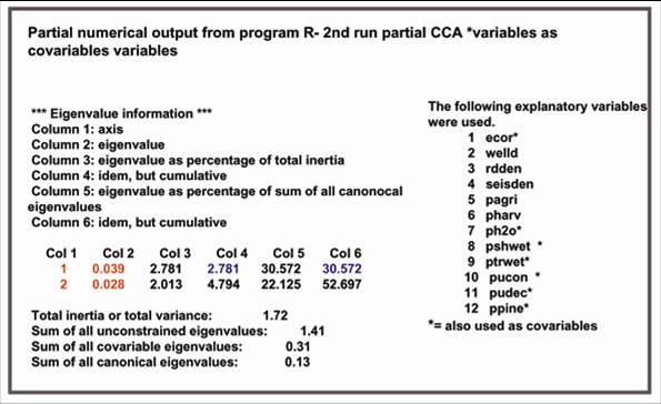
In order to partition the variance that could be explained by disturbance variables vs habitat variables I tested two other multivariate techniques: partial CCA and partial RDA(3). While these analyses each assume a unimodal response or linear response of the species respectively, each allows for variables to be included as covariates. Like regular CCA and RDA, both techniques are considered types of direct gradient analysis - the final configuration of the ordination diagram is constrained by the environmental variables included in the analysis (3). They also assume that all the important variables have been measured and that the environmental data are normally distributed (4). In a preliminary ordination, the total gradient length of the analyses for the first axis was 2.5. A gradient length of more than 3 s.d suggests unimodal response of the species data, while a gradient length of less than 2.0 s.d. suggests a linear analysis is more appropriate 3. My result of 2.5 s.d. represents a grey zone in multivariate analysis for choosing between linear and unimodal techniques where either analysis is expected to provide a similar configuration. Thus, both approaches were tested. Both yielded eigenvalues for the first ordination axis under 0.5 suggesting a poor separation of species along an ordination axis (3). The diagrams produced did reflect general trends observed in NMS (Main Text) however given the limitations of the numerical output (Fig. 1) I deemed them unreliable. Results were similar for both raw data and log-transformed data.( log (x+1)).

a.)	b.)
Fig 1. A sample numerical output from “Program R” demonstrating the limitations of using CCA/RDA for my data. a.) A CCA output performed using all variables remaining after eliminating collinear variables. b.) Output from partial CCA using habitat variables as covariables and only the disturbance variables as explanatory variables. Some explanatory remarks are included in the figure.

Data Preparation

A number of data preparation steps were necessary including spatial analysis and exploratory data analyisis.

Spatial Analysis: I conducted spatial analyses to calculate the amount of disturbance and proportion of each of the habitat variables in each block and around each wetland surveyed within the blocks. I used a nested buffer approach for the wetland scale work. Using ArcGis or ArcView 3.2 (depending on the dataset-and technical glitches) I tabulated the disturbance values as well as the habitat attributes at 100m, 200m 500m and 1000m scales. I chose these scales based on other studies in the literature that used the nested buffer approach (5;6) as well as based on thelimitations of the 30 m resolution of the satellite imagery. In addition, for some blocks I did no have a remotely sensed habitat inventory that covered all blocks so I had to use 2 different sources the Alberta Ground Cover Classification and the Alberta Woodlot inventory to manually derive classes of similar value to those in the Ducks Unlimited Enhanced Wetland Classification used in the remainder of the blocks This was time consuming at the 5 x 5 km scale (2 days for 6 blocks). and thus became unfeasible to derive these classes for the individual buffers (35-45 buffers at each scale) for this project. This problem was biased for the agricultural sites for which I could calculate disturbance values but not other habitat attributes. The values that were available were added into a relational data base.

Exploring the data: I examined the data to see whether parametric or nonparametric methods should be applied. Kolmgornov-Smirnov tests revealed that all variables were non-normal. Though the distribution for species could not be adjusted through tranformation, a log transformation log (X+1) was applied to equalize the weights in multivariate analysis of common and uncommon species(3,4). For proportional habitat variables an Arcsine tranformation was applied (4). Distribution of some of the habitat variables can be examined here. I performed an oulier analyis also. One block was found to be an outlier due to an unsually high count of American Avocets. This count was eliminated from the data as it only occurred at one wetland. The block remained part of the complete data set.

Establishing Groups: For each type of disturbance including total disturbance an a priori set of groupings was developed to faciltate categorical analysis of community data using disturbances independently. I did this at both a wetland and block scale although only block data are presented. Not all blocks were used in each category. For example no blocks had both agriculture and harvesting. Many blocks also had a high total disturbance and could not be used as a reference block despite not having the disturbance for which the category was being established. The sample size for each group is listed in the analysis or in the figure wherever approrpiate..Groups were as follows:

*The Cumulative Effects Index or CEI was calculated prior to data collection for the whole landscape in order to select sites. A roving window analysis was used to calculate total amount of disturbance by type in a 5 km X 5 km block at 200 m intervals resulting in a base sample of 200,000 blocks. Each block is then ranked for each disturbance within the entire set of possible blocks. The rank is divided by the total possible ranks (0's are assigned a value of 0) which returns a value between 0 and 1. The CEI is the sum of these ranks and applies no weigthing to any particular disturbance. The procedure was developed by Dr. E. Bayne as part of the Integrated Landscape Mangement Project at the University of Alberta.

I used 4 main statistical programs to analyze data:

STATA Version 8.0. Exploratory data analysis, summary statistics and graphs of explanatory variables, curve fitting.

PC-Ord Version 4.0 - Exploratory analysis using a range of ordination techniques, outlier analysis, and MRPP.

Program R – partial CCA and RDA; db-MRT’s – I used Brodgar or code to conduct the analysis

PRIMER- Version 5. MVDISP, SIMPER procedures described in Main Text.

Reference List