Ch E 416 - Assignment 2 Solutions
Problem 1
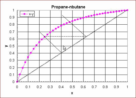
(2.1) Graphical technique
The mass
balance eqn is y=(y-1)/y x + Zf/ y with y =0.4 and the feed to stage 1 is Zf=0.4.
When x=0.2, y=0.7 from the mass balance equation.
Draw a line through (0.4,0.4) and (0.2,0.7).
Outlet
compositions are (0.25,0.63).
The feed to
stage 2 is Zf=0.63. The mass balance eqn is y=(y-1)/y x + Zf/ y with y =0.4
When x=0.5, y=0.8 from the mass balance equation.
Draw a line through (0.63,0.63) and (0.5,0.8).
Outlet
compositions are (0.47,0.83).
(2.2) Analytical solution
Solve the two equations
y= 5.44x/(1+4.44x) and y=-1.5x + 1
simultaneously for (x,y)
In MATLAB you can solve these by
using a single line
>>[x,y]=solve('y=1-1.5*x','y=5.44*x/(1+4.44*x)')
It
produces the result
x =
[
-.61824177053872876301043257229182]
[ .24286639516335338763505719691644]
y =
[
1.9273626558080931445156488584377]
[ .63570040725496991854741420462533]
Hence
the desired result is (0.2429,0.6357).
For
the second stage the two equations are
y= 5.44x/(1+4.44x) and y=-1.5x +
0.6357/0.4
>>
[x,y]=solve('y=0.6357/0.4-1.5*x','y=5.44*x/(1+4.44*x)')
x =
[
-.47984273653486611514443863085348]
[
.49730069449282407310239658881143]
y =
[
2.3090141048022991727166579462802]
[ .84329895826076389034640511678285]
Hence
the desired result is (0.4973,0.8432).
(2.3) MATLAB solution
The MATLAB function to solve this
problem is here (A2_P2_f.m). The functions to
calculate fugacities are included in the same m
file as sub-functions. You can delete them and use the fugacity functions you
used for assignment 1 if you so wish.
The MATLAB script you need to
solve the function is here (A2_P2.m).
Reproduced below:
xx0 = [.5 .5 .5 .5 250 .5 .5 .5 .5 230]';
xx=fsolve('A2_P2_f',xx0,options);
x3 = xx(1:2);
y2 = xx(3:4);
T2 = xx(5)-273.15;
x4 = xx(6:7);
y5 = xx(8:9);
T4 = xx(10)-273.15;
Stage1_xyT = [x3 y2 T2*ones(2,1)]
Stage2_xyT = [x4 y5 T4*ones(2,1)]
Norm
of First-order Trust-region
Iteration
Func-count f(x) step optimality radius
0
11 0.54752 1.19 1
1
22 0.199925 1 0.255 1
2
33 0.0842315 2.5 0.269 2.5
3
44 0.0166742 6.25 0.0564 6.25
4
55 7.27311e-005 6.22425 0.011 15.6
5
66 1.43092e-009 0.308175 6.15e-005 15.6
6
77 5.34676e-019 0.00116314 1.24e-009 15.6
7
88 2.32421e-030 2.23793e-008 2.49e-015 15.6
Optimization
terminated: first-order optimality is less than options.TolFun.
Stage1_xyT =
0.2505
0.6243 -18.0767
0.7495
0.3757 -18.0767
Stage2_xyT =
0.4829
0.8363 -28.3858
0.5171
0.1637 -28.3858
Note that the temperature is in
deg C.
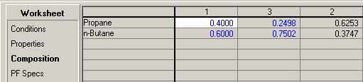
(2.4) HYSYS simulation
The HYSYS simulation file is A2_Hysys.hsc Notice that in HYSYS you need a cooler
between the two flash stages to condense part of the
vapour.
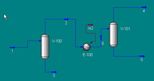
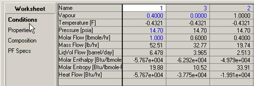
The
results from HYSYS are shown below.
Block
V-100
Block
V-101
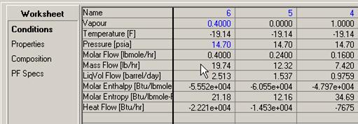
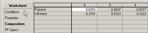
Notice that the results get
progressively more accurate.
Posted September 29, 2006
Return
to Assignments Page
|