Plane-Wave Solutions

We have already solved the Dirac equation for free particles at rest. The Lorentz transformation may be used to construct the free-particle solutions for an arbitrary velocity.

It is easy to see the invariant form of the exponential by writing its form in the rest frame of the particle

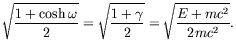
$$\exp (-i\epsilon_r p\cdot x/\hbar) \rightarrow \exp (-i\epsilon_r Et/\hbar) \rightarrow \exp (-i\epsilon_r mc^2t/\hbar) ,$$ (5.179)

where $r=1,2,3,4$, and $\epsilon_r=+1$ for $r=1,2$ and $\epsilon_r=-1$ for $r=2,3$. The positive-energy solutions ($r=1,2$) and negative-energy solutions ($r=3,4$) transform among themselves separately and do not mix with each other under proper Lorentz transformations, as well as, under spatial inversions.

For a Lorentz transformation of a particle from rest ( $\hat{v} = -\vec{p}/\vert\vec{p}\vert$)

$$\beta = \frac{pc}{E} \quad\textrm{and}\quad \gamma = \frac{E}{mc^2}.$$ (5.180)

Using (3.17) and (3.18) we can thus write

$$\tanh\frac{\omega}{2} = \frac{\sinh\omega}{1+\cosh\omega} = \frac{\gamma\beta}{1+\gamma} = \frac{pc}{E+mc^2} ,$$ (5.181)

$$\cosh\frac{\omega}{2} = \sqrt{\frac{1+\cosh\omega}{2}} = \sqrt{\frac{1+\gamma}{2}} = \sqrt{\frac{E+mc^2}{2mc^2}} .$$ (5.182)

To calculate the Lorentz transformation matrix, $S$, we will need

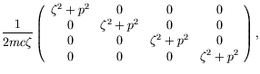
$$\vec{p}\cdot\vec{\sigma} =\left(\begin{array}{cc} 0 & p_x \... ...y}{cc} p_z & p_x-ip_y \\ p_x+ip_y & -p_z \end{array}\right) .$$ (5.183)

Using this results with (5.147) gives

$$S = \sqrt{\frac{E+mc^2}{2mc^2}} \left[ \begin{array}{cccc} 1 & 0 & \f... ...& 0 \\ \frac{p_+c}{E+mc^2} & \frac{-p_zc}{E+mc^2} & 0 & 1 \end{array} \right],$$ (5.184)

where $p_{\pm} = p_x\pm ip_y$. From (5.18) and (5.19), we see that each of the four general solutions to the Dirac equation correspond to one of the columns of the above transformation matrix.

Let us now look at some of the properties of the general solution to the Dirac equation. The general form of the wave function is

$$\psi^r(x) = w^r(\vec{p})e^{-i\epsilon_rp\cdot x/\hbar} .$$ (5.185)

Substitution into the Dirac equation gives

$$\left( i\hbar \frac{\partial}{\partial x_\mu} \gamma_\mu - mc \right) \omega^r(\vec{p})e^{-i\epsilon_rp\cdot x/\hbar} = 0$$

$$\left( i\hbar \frac{-i\epsilon_rp^\mu}{\hbar} \gamma_\mu - mc \right) \omega^r(\vec{p}) = 0$$

$$(\epsilon_r \not{\!p} - mc ) \omega^r(\vec{p}) = 0 ,$$ (5.186)

$$\fbox{$\displaystyle (\not{\!p} - \epsilon_rmc ) \omega^r(\vec{p}) = 0 $}\ ,$$ (5.187)

which is the Dirac equation in momentum space. The adjoint equation is

$$\psi^{\dagger r}(x)\left(-i\hbar \frac{\stackrel{\leftarrow}{\partial}}{\partial x_\mu} \gamma^\dagger_\mu - mc \right) = 0$$

$$\omega^r(\vec{p})^\dagger e^{i\epsilon_rp\cdot x/\hbar} \left(-i\... ...stackrel{\leftarrow}{\partial}}{\partial x_\mu} \gamma^\dagger_\mu - mc \right) = 0$$

$$\overline{\omega}^r(\vec{p})\gamma_0\left( -i\hbar \frac{i\epsilon_rp^\mu}{\hbar} \gamma^\dagger_\mu - mc \right) = 0$$

$$\overline{\omega}^r(\vec{p})\left( \epsilon_rp^\mu\gamma_0\gamma^\dagger_\mu\gamma_0 - mc \right) = 0$$

$$\overline{\omega}^r(\vec{p})(\epsilon_r\not{\!p} - mc ) = 0$$

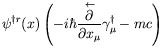$$\overline{\omega}^r(\vec{p})(\not{\!p} -\epsilon_r mc ) = 0 .$$ (5.188)

Since the covariant normalization statement

$$\overline{\omega}^r(\vec{p})\omega^{r\prime}(\vec{p})$$ (5.189)

is a Lorentz scalar we may evaluate it in the rest frame for simplicity.

$$\overline{\omega}^r(\vec{p})\omega^{r\prime}(\vec{p}) = \ove... ...)\gamma_0\omega^{r\prime}(0) = \epsilon_r\delta_{rr^\prime} .$$ (5.190)

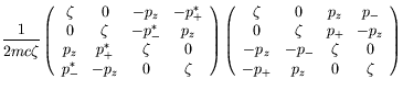
The completeness relationship is

$$\sum_{r=1}^4 \epsilon_r w^r_\alpha(\vec{p}) \overline{w}^r_\beta(\vec{p}).$$ (5.191)

We first evaluate it in the rest frame and then boost to the moving frame. For a particle at rest

$$\omega^r(0)\overline{\omega}^r(0) = \omega^r(0)\omega^{r\dag... ... & -1 \end{array} \right) \quad\textrm{for}\ r=4 . \end{array}$$

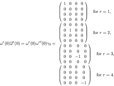Therefore

$$\sum^4_{r=1}\epsilon_r\omega^r(0)\overline{\omega}^r(0) = I ... ...alpha(0)\overline{\omega}^r_\beta(0) = \delta_{\alpha\beta} .$$ (5.192)

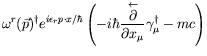
For a particle in motion

$$\sum^4_{r=1} \epsilon_r \omega^r_\alpha(\vec{p}) \overline{\omega}^r_\beta(\vec{p}) = \sum^4_{r=1} \epsilon_r S_{\alpha\gamma}\left(\frac{-\vec{p}c}{E}... ...line{\omega}^r_\lambda(0) S_{\lambda\beta}^{-1}\left(\frac{-\vec{p}c}{E}\right)$$

$$= S_{\alpha\gamma}\left(\frac{-\vec{p}c}{E}\right) \delta_{\gamma\lambda} S_{\lambda\beta}^{-1}\left(\frac{-\vec{p}c}{E}\right)$$

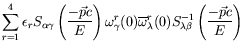$$= \delta_{\alpha\beta} .$$ (5.193)

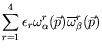
The probability density

$$\omega^{r\dagger} (\epsilon_r\vec{p}) \omega^{r^\prime} (\epsilon_{r^\prime}\vec{p})$$ (5.194)

will not be an invariant but transforms as the zeroth component of a vector. Boosting the particle at rest we have

$$\omega^{r\dagger}(\epsilon_r\vec{p}) \omega^{r^\prime}(\epsi... ...n_{r^\prime}\vec{p}c}{E}\right) \omega^{r^\prime}_\delta(0) .$$ (5.195)

Defining $\zeta = (E+mc^2)/c$ and noticing that $p_+^*=p_-; p_-^*=p_+; p_+p_+^*=p_x^2+p_y^2;p_-p_-^*=p_x^2+p_y^2$, we calculate

$$S^\dagger\left(\frac{-\epsilon_r\vec{p}}{E}\right) S\left(\frac{-\epsilon_{r^\prime}\vec{p}}{E}\right)$$

$$= \frac{1}{2mc\zeta} \left( \begin{array}{cccc} \zeta & 0 & -p_z & ... ...-p_z \\ -p_z & -p_- & \zeta & 0 \\ -p_+ & p_z & 0 & \zeta \end{array} \right)$$

$$= \frac{1}{2mc\zeta} \left( \begin{array}{cccc} \zeta^2+p_z^2+p_+p_... ...eta-p_+\zeta & 0 & p_zp_-^*-p_zp_+ & p_-p_-^*+p_z^2+\zeta^2 \end{array} \right)$$

$$= \frac{1}{2mc\zeta} \left( \begin{array}{cccc} \zeta^2+p^2 & 0 & 0... ...0 \\ 0 & 0 & \zeta^2+p^2 & 0 \\ 0 & 0 & 0 & \zeta^2+p^2 \end{array} \right) ,$$ (5.196)

$$\omega^{r\dagger}(\epsilon_r\vec{p}) \omega^{r^\prime}(\epsilon_{r^\prime}\vec{p}) = \frac{E}{mc^2} \delta_{rr^\prime} .$$ (5.197)